Code
from utils import Float, Array, Callable, plt, np, latex
from torchvision.datasets import MNIST
from config import MNIST_PATHfrom utils import Float, Array, Callable, plt, np, latex
from torchvision.datasets import MNIST
from config import MNIST_PATHSupervised learning (SL) is a core subfield of machine learning alongside RL and unsupervised learning. The typical SL task is to approximate an unknown function given a dataset of input-output examples from that function.
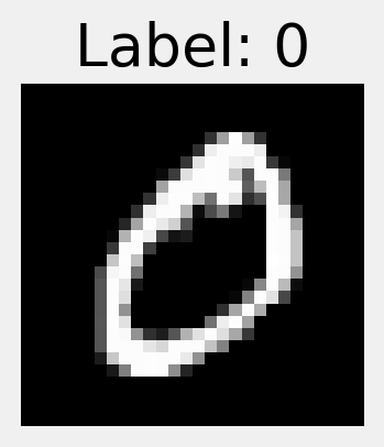
Example 5.1 (Image classification) One of the most common examples of an SL problem is the task of image classification: Given a dataset of images and their respective labels, construct a function that takes an image and outputs the correct label.
fig. 5.1 illustrates two samples (that is, input-output pairs) from the MNIST database of handwritten digits (Deng, 2012). This is a task that most humans can easily accomplish. By providing many samples of digits and their labels to a machine, SL algorithms can learn to solve this task as well.
data = MNIST(MNIST_PATH, train=True, download=True)

plt.figure(figsize=(2, 2))
plt.axis('off')
plt.imshow(data.data[0], cmap='gray')
# plt.title(f"Label: {data.targets[0]}")
plt.show()

plt.figure(figsize=(2, 2))
plt.axis('off')
plt.imshow(data.data[1], cmap='gray')
# plt.title(f"Label: {data.targets[1]}")
plt.show()
When might function approximation be useful in RL? Recall that the definition of an MDP includes the state transitions \(P : \mathcal{S} \times \mathcal{A} \to \triangle(\mathcal{S})\) and a reward function \(r : \mathcal{S} \times \mathcal{A} \to \mathbb{R}\) (def. 2.4). If we know both of these functions, in the sense that we are able to query them on arbitrary inputs, we can use powerful planning algorithms to solve for the optimal policy exactly (see Section 2.3.2). Thus, if either (or both) of these is not known, we can use an SL algorithm to model the environment and then solve the modeled environment using dynamic programming. This approach is called fitted DP and will be covered in Chapter 6.
We do not seek to comprehensively discuss supervised learning; see the bibiographic notes at the end of the chapter (Section 5.6) for further resources. We hope to to leave you with an understanding of what types of problems SL can solve and how SL algorithms can be applied to RL.
In SL, we are given a dataset of labelled samples \((x_1, y_1), \dots, (x_N, y_N)\) that are independently sampled from some data generating process. Mathematically, we describe this data generating process as a joint distribution \(p \in \triangle(\mathcal{X} \times \mathcal{Y})\), where \(\mathcal{X}\) is the space of possible inputs and \(\mathcal{Y}\) is the space of possible outputs. Note that, by the chain rule of probability, this can be factored as \(p(x, y) = p(y \mid x) p(x)\).
Example 5.2 (Joint distributions for image classification) For example, in ex. 5.1, the marginal distribution over \(x\) is assumed to be the distribution of handwritten digits by humans, scanned as \(28 \times 28\) grayscale images. The conditional distribution \(y \mid x\) is assumed to be the distribution over \(\{ 0, \dots, 9 \}\) that a human would assign to the image \(x\).
Our task is to compute a “good” prediction rule \(\hat f : \mathcal{X} \to \mathcal{Y}\) that takes an input and tries to predict the corresponding output.
How can we measure how “good” a prediction rule is? The most common way is to use a loss function \(\ell : \mathcal{Y} \times \mathcal{Y} \to \mathbb{R}\) that compares the guess \(\hat y := \hat f(x)\) with the true output \(y\). \(\ell(\hat y, y)\) should be low if the prediction rule accurately guessed the output, and high if the prediction was incorrect.
Example 5.3 (Zero-one loss) In the image classification task ex. 5.1, we have \(X = [0, 1]^{28 \times 28}\) (the space of \(28\)-by-\(28\) grayscale images) and \(Y = \{ 0, \dots, 9 \}\) (the image’s label). We could use the zero-one loss function,
\[ \ell(\hat y, y) = \begin{cases} 0 & \hat y = y \\ 1 & \hat y \ne y \end{cases} \tag{5.1}\]
to measure the accuracy of the prediction rule. That is, if the prediction rule assigns the wrong label to an image, it incurs a loss of one for that sample.
Example 5.4 (Square loss) For a continuous output (i.e. \(\mathcal{Y} \subseteq \mathbb{R}\)), we typically use the squared difference as the loss function:
\[ \ell(\hat y, y) = (\hat y - y)^2 \tag{5.2}\]
The square loss is nice to work with analytically since its derivative with respect to \(\hat y\) is simply \(2 (\hat y - y)\). (Sometimes authors define the square loss as half of the above value to cancel the factor of \(2\) in the derivative. Generally speaking, scaling the loss by some constant scalar has no practical effect.)
x = np.linspace(-1, 1, 20)
y = x ** 2
plt.plot(x, y)
plt.xlabel(r"$\hat y - y$")
plt.ylabel(r"$\ell(\hat y, y)$")
plt.show()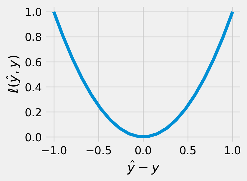
Ultimately, we want a prediction rule that does well on new, unseen samples from the data generating process. We can thus ask, how much loss does the prediction rule incur in expectation? This is called the prediction rule’s generalization error or test error.
Definition 5.1 (Generalization error) Given a loss function \(\ell\) and a prediction rule \(\hat f\), the generalization error of the prediction rule is defined as the expected loss over the data generating process.
\[ \text{error}_{\text{g}}(\hat f) := \mathop{\mathbb{E}}_{(x, y) \sim p} [ \ell(\hat f(x), y) ] \tag{5.3}\]
Suppose we sample a new input and output from the data generating process, make a guess according to our prediction rule, and use the loss function to compare our guess to the true output. If we repeat this many times, the average loss would approach the generalization error.
The goal of SL is then to find the prediction rule that minimizes the test error. For certain loss functions, the theoretical optimum can be analytically computed, such as for squared error.
Theorem 5.1 (The conditional expectation minimizes mean squared error) An important result is that, under the square loss, the optimal prediction rule is the conditional expectation:
\[ \arg\min_{f} \mathop{\mathbb{E}}[(y - f(x))^2] = (x \mapsto \mathop{\mathbb{E}}[y \mid x]) \tag{5.4}\]
Proof. We can decompose the mean squared error as
\[ \begin{aligned} \mathop{\mathbb{E}}[(y - f(x))^2] &= \mathop{\mathbb{E}}[ (y - \mathop{\mathbb{E}}[y \mid x] + \mathop{\mathbb{E}}[y \mid x] - f(x))^2 ] \\ &= \mathop{\mathbb{E}}[ (y - \mathop{\mathbb{E}}[y \mid x])^2 ] + \mathop{\mathbb{E}}[ (\mathop{\mathbb{E}}[y \mid x] - f(x))^2 ] \\ &\quad {} + 2 \mathop{\mathbb{E}}[ (y - \mathop{\mathbb{E}}[y \mid x])(\mathop{\mathbb{E}}[y \mid x] - f(x)) ] \\ \end{aligned} \tag{5.5}\]
We leave it as an exercise to show that the last term is zero. (Hint: use the law of iterated expectations.) The first term is the noise, or irreducible error, that doesn’t depend on \(f\), and the second term is the error due to the approximation, which is minimized at \(0\) when \(f(x) = \mathop{\mathbb{E}}[y \mid x]\).
In most applications, such as in ex. 5.2, we can’t integrate over the joint distribution of \(x, y\), and so we can’t evaluate \(\mathop{\mathbb{E}}[y \mid x]\) analytically. Instead, all we get are \(N\) samples from the joint distribution of \(x\) and \(y\). How might we use these to approximate the generalization error?
To estimate the generalization error, we could simply take the sample mean of the loss over the training data. This is called the training loss or empirical risk:
Definition 5.2 (Empirical risk) Given a dataset \((x_1, y_1), \dots, (x_N, y_N)\) sampled i.i.d. from the data generating process, and a loss function \(\ell\), the empirical risk of the prediction rule \(\hat f\) is the average loss across the dataset:
\[ \text{training loss}(\hat f) := \frac 1 N \sum_{n=1}^N \ell(\hat f(x_n), y_n). \tag{5.6}\]
By the law of large numbers, as \(N\) grows to infinity, the training loss converges to the generalization error (def. 5.1).
The empirical risk minimization (ERM) approach is to find a prediction rule that minimizes the empirical risk.
Definition 5.3 (Empirical risk minimization) An ERM algorithm requires two ingredients to be chosen based on our domain knowledge about the DGP:
This allows us to compute the empirical risk minimizer:
\[ \begin{aligned} \hat f_\text{ERM} &:= \arg\min_{f \in \mathcal{F}} \text{training loss}(f) \\ &= \arg\min_{f \in \mathcal{F}}\frac 1 N \sum_{n=1}^N \ell(f(x_n), y_n). \end{aligned} \tag{5.7}\]
How should we choose the correct function class? In fact, why do we need to constrain our search at all?
Exercise 5.1 (Overfitting) Suppose we are trying to approximate a relationship between real-valued inputs and outputs using square loss as our loss function. Consider the prediction rule (visualized in fig. 5.3)
\[ \hat f(x) = \sum_{n=1}^N y_n \mathbf{1}\left\{x = x_n\right\}. \tag{5.8}\]
What is the empirical risk of this function? How well does it perform on newly generated samples?
n = 1000
x_axis = np.linspace(-1, +1, n)

for _ in range(2):
    x_train = np.random.uniform(-1, +1, 10)
    y_train = np.sin(np.pi * x_train)
    y_hat = np.where(np.isclose(x_axis[:, None], x_train, atol=2/n), y_train, 0).sum(axis=-1)

    plt.plot(x_axis, y_hat, label=r'$\hat f(x)$')
    plt.scatter(x_train, y_train, color='red', marker='x', label='training data')
    plt.legend()
    plt.gcf().set_size_inches(3, 2)
    plt.show()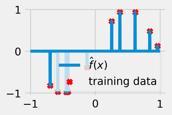
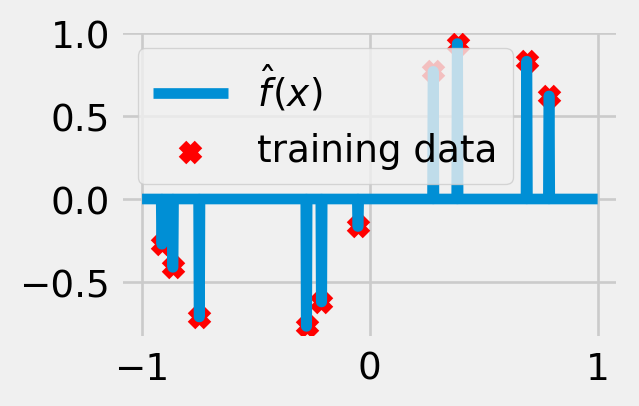
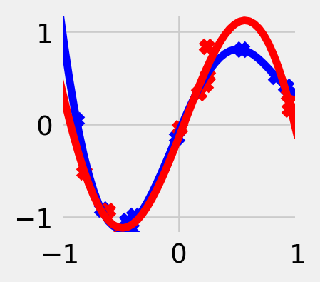
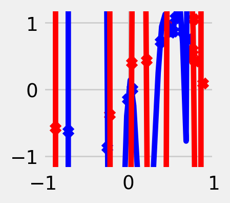
The choice of \(\mathcal{F}\) depends on our domain knowledge about the task. On one hand, \(\mathcal{F}\) should be large enough to contain the true relationship, but on the other, it shouldn’t be too expressive; otherwise, it will overfit to random noise in the labels. The larger and more complex the function class, the more accurately we will be able to approximate any particular training dataset (i.e. smaller bias), but the more drastically the function will vary for different training datasets (i.e. larger variance). For most loss functions, including the square loss, it is possible to express the generalization error (def. 5.1) as a sum of a bias term and a variance term. The mathematical details of this so-called bias-variance tradeoff can be found, for example, in Hastie et al. (2013, Chapter 2.9).
n_samples = 10
degrees = [2, 5, 50]
x_axis = np.linspace(-1, +1, 50)


def generate_data(sigma=0.2):
    x_train = np.random.uniform(-1, +1, n_samples)
    y_train = np.sin(np.pi * x_train) + sigma * np.random.normal(size=n_samples)
    return x_train, y_train


def transform(x: Float[Array, " N"], d: int):
    return np.column_stack([
        x ** d_
        for d_ in range(d + 1)
    ])


for d in degrees:
    for _ in range(2):
        x_train, y_train = generate_data()

        x_features = transform(x_train, d)
        w = np.linalg.lstsq(x_features, y_train)[0]
        y_hat = transform(x_axis, d) @ w

        color = 'blue' if _ == 0 else 'red'
        plt.scatter(x_train, y_train, color=color, marker='x')
        plt.plot(x_axis, y_hat, color=color)
    plt.xlim(-1, +1)
    plt.ylim(-1.2, 1.2)
    plt.gcf().set_size_inches(2, 2)
    plt.show()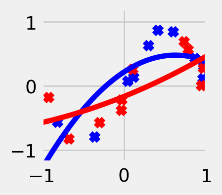
We must also consider practical constraints on the function class. We need an efficient algorithm to actually compute the function in the class that minimizes the training error. This point should not be underestimated! The success of modern deep learning, for example, is in large part due to hardware developments that have made certain operations more efficient than others.
Both of the function classes we will consider, linear maps and neural networks, are finite-dimensional, a.k.a. parameterized. The notion of a parameterized function class is best illustrated by example:
Example 5.5 (Quadratic functions) consider the class of quadratic functions, i.e. polynomials of degree \(2\). This is a three-dimensional function space (\(D = 3\)), since we can describe any quadratic \(p\) as
\[ p(x) = a x^2 + b x + c, \tag{5.9}\]
where \(a, b, c\) are the three parameters. We could also use a different parameterization:
\[ p(x) = a' (x - b')^2 + c'. \tag{5.10}\]
Definition 5.4 (Parameters) Let \(\mathcal{F}\) be a class of functions mapping from \(\mathcal{X}\) to \(\mathcal{Y}\). We say that \(\mathcal{F}\) is a parameterized function class if each \(f \in \mathcal{F}\) can be identified using \(D\) parameters.
Exercise 5.2 (Parameterization matters) Note that the choice of parameterization can impact the performance of the chosen fitting method. What is the derivative of eq. 5.9 with respect to \(a, b, c\)? Compare this to the derivative of eq. 5.10 with respect to \(a', b', c'\). This shows that gradient-based fitting methods may change their behaviour depending on the parameterization.
Using a parameterized function class allows us to reframe the ERM problem def. 5.3 in terms of optimizing over the parameters instead of over the functions they represent:
\[ \begin{aligned} \hat \theta_\text{ERM} &:= \arg\min_{\theta \in \mathbb{R}^D} \text{training loss}(f_\theta) \\ &= \frac{1}{N} \sum_{n=1}^N (y_n - f_\theta(x_n))^2 \end{aligned} \tag{5.11}\]
In general, optimizing over a finite-dimensional space is much, much easier than optimizing over an infinite-dimensional space.
One widely applicable fitting method for parameterized function classes is gradient descent.
Let \(L(\theta) = \text{training loss}(f_\theta)\) denote the empirical risk in terms of the parameters. The gradient descent algorithm iteratively updates the parameters according to the rule
\[ \theta^{t+1} = \theta^t - \eta \nabla_\theta L(\theta^t) \]
where \(\eta > 0\) is the learning rate and \(\nabla_\theta L(\theta^t)\) indicates the gradient of \(L\) at the point \(\theta^t\). Recall that the gradient of a function at a point is a vector in the direction that increases the function’s value the most within a neighborhood. So by taking small steps in the oppposite direction, we obtain a solution that achieves a slightly lower loss than the current one.
Params = Float[Array, " D"]


def gradient_descent(
    loss: Callable[[Params], float],
    θ_init: Params,
    η: float,
    epochs: int,
):
    """
    Run gradient descent to minimize the given loss function
    (expressed in terms of the parameters).
    """
    θ = θ_init
    for _ in range(epochs):
        θ = θ - η * grad(loss)(θ)
return θIn Section 7.3.1, we will discuss methods for implementing the grad function above, which takes in a function and returns its gradient, which can then be evaluated at a point.
Why do we need to scale down the step size by \(\eta\)? The key word above is “neighborhood”. The gradient only describes the function within a local region around the point, whose size depends on the function’s smoothness. If we take a step that’s too large, we might end up with a worse solution by overshooting the region where the gradient is accurate. Note that, as a result, we can’t guarantee finding a global optimum of the function; we can only find local optima that are the best parameters within some neighborhood.
Another issue is that it’s often expensive to compute \(\nabla_\theta L\) when \(N\) is very large. Instead of calculating the gradient for every point in the dataset and averaging these, we can simply draw a batch of samples from the dataset and average the gradient across just these samples. Note that this is an unbiased random estimator of the true gradient. This algorithm is known as stochastic gradient descent. The added noise sometimes helps to jump to better solutions with a lower overall empirical risk.
Stepping for a moment back into the world of RL, you might wonder, why can’t we simply apply gradient descent to the total reward? It turns out that the gradient of the total reward with respect to the policy parameters known as the policy gradient, is challenging but possible to approximate. In Chapter 7, we will do exactly this.
In linear regression, we assume that the function \(f\) is linear in the parameters:
\[ \mathcal{F} = \{ x \mapsto \theta^\top x \mid \theta \in \mathbb{R}^D \} \]
You may already be familiar with linear regression from an introductory statistics course. This function class is extremely simple and only contains linear functions, whose graphs look like “lines of best fit” through the training data. It turns out that, when minimizing the squared error, the empirical risk minimizer has a closed-form solution, known as the ordinary least squares estimator. Let us write \(Y = (y_1, \dots, y_n)^\top \in \mathbb{R}^N\) and \(X = (x_1, \dots, x_N)^\top \in \mathbb{R}^{N \times D}\). Then we can write
\[ \begin{aligned} \hat \theta &= \arg\min_{\theta \in \mathbb{R}^D} \frac{1}{2} \sum_{n=1}^N (y_n - \theta^\top x_n)^2 \\ &= \arg\min_{\theta \in \mathbb{R}^D} \frac 1 2 \|Y - X \theta \|^2 \\ &= (X^\top X)^{-1} X^\top Y, \end{aligned} \tag{5.12}\]
where we have assumed that the columns of \(X\) are linearly independent so that the matrix \(X^\top X\) is invertible.
What happens if the columns aren’t linearly independent? In this case, out of the possible solutions with the minimum empirical risk, we typically choose the one with the smallest norm.
Exercise 5.3 (Gradient descent finds the minimum norm solution) Gradient descent on the ERM problem (eq. 5.12), initialized at the origin and using a small enough step size, eventually finds the parameters with the smallest norm. In practice, since the squared error gradient is convenient to compute, running gradient descent can be faster than explicitly computing the inverse (or pseudoinverse) of a matrix.
Assume that \(N < D\) and that the data points are linearly independent.
Let \(\hat{\theta}\) be the solution found by gradient descent. Show that \(\hat{\theta}\) is a linear combination of the data points, that is, \(\hat{\theta} = X^\top a\), where \(a \in \mathbb{R}^N\).
Let \(w \in \mathbb{R}^D\) be another empirical risk minimizer i.e. \(X w = y\). Show that \(\hat{\theta}^\top (w - \hat{\theta}) = 0\).
Use this to show that \(\|\hat{\theta}\| \le \|w\|\), showing that the gradient descent solution has the smallest norm out of all solutions that fit the data. (No need for algebra; there is a nice geometric solution!)
Though linear regression may appear trivially simple, it is a very powerful tool for more complex models to build upon. For instance, to expand the expressiveness of linear models, we can first transform the input \(x\) using some feature mapping \(\phi\), i.e. \(\widetilde x = \phi(x)\), and then fit a linear model in the transformed space instead. By using domain knowledge to choose a useful feature mapping, we can obtain a powerful SL method for a particular task.
In neural networks, we assume that the function \(f\) is a composition of linear functions (represented by matrices \(W_i\)) and non-linear activation functions (denoted by \(\sigma\)):
\[ \mathcal{F} = \{ x \mapsto \sigma(W_L \sigma(W_{L-1} \dots \sigma(W_1 x + b_1) \dots + b_{L-1}) + b_L) \} \]
where \(W_\ell \in \mathbb{R}^{D_{\ell+1} \times D_\ell}\) and \(b_\ell \in \mathbb{R}^{D_{\ell+1}}\) are the parameters of the \(i\)-th layer, and \(\sigma\) is the activation function.
This function class is highly expressive and allows for more parameters. This makes it more susceptible to overfitting on smaller datasets, but also allows it to represent more complex functions. In practice, however, neural networks exhibit interesting phenomena during training, and are often able to generalize well even with many parameters.
Another reason for their popularity is the efficient backpropagation algorithm for computing the gradient of the output with respect to the parameters. Essentially, the hierarchical structure of the neural network, i.e. computing the output of the network as a composition of functions, allows us to use the chain rule to compute the gradient of the output with respect to the parameters of each layer.
Supervised learning is a field of machine learning that seeks to approximate some unknown function given a dataset of example input-output pairs from that function. In particular, we typically seek to compute a prediction rule that takes in an input value and returns a good guess for the corresponding output. We score prediction rules using a loss function that measures how incorrectly it guesses. We want to find a prediction rule that achieves low loss on unseen data points. We do this by searching over a class of functions to find one that minimizes the empirical risk over the training dataset. We finally saw two popular examples of parameterized function classes: linear regression and neural networks.
Supervised learning is the largest subfield of machine learning; we do not attempt to comprehensively survey recent progress here. Rather, here are some textbooks for interested students to read further.
James et al. (2023) provides an accessible introduction to supervised learning. Hastie et al. (2013) examines the subject in even further depth and covers many relevant supervised learning methods. Nielsen (2015) provides a comprehensive introduction to neural networks and backpropagation. Vapnik (2000) is another prominent textbook on classical statistical learning from before the “deep learning era”. Bishop (2006) focuses on the Bayesian perspective.