4 Multi-Armed Bandits

4.1 Introduction

The multi-armed bandit (MAB) problem is a simple setting for studying the basic challenges of sequential decision-making. In this setting, an agent repeatedly chooses from a fixed set of actions, called arms, each of which has an associated reward distribution. The agent’s goal is to maximize the total reward it receives over some time period. Here are a few examples:

Example 4.1 (Online advertising) Let’s suppose you, the agent, are an advertising company. You have $K$ different ads that you can show to users. Let’s suppose you are targeting a single user. You receive $1$ reward if the user clicks the ad, and $0$ otherwise. Thus, the unknown reward distribution associated to each ad is a Bernoulli distribution defined by the probability that the user clicks on the ad. Your goal is to maximize the total number of clicks by the user.

Deciding which ad to put on a billboard can be treated as a MAB problem. Image from Negative Space (2015).

Example 4.2 (Clinical trials) Suppose you’re a pharmaceutical company, and you’re testing a new drug. You have $K$ different dosages of the drug that you can administer to patients. You receive $1$ reward if the patient recovers, and $0$ otherwise. Thus, the unknown reward distribution associated with each dosage is a Bernoulli distribution defined by the probability that the patient recovers. Your goal is to maximize the total number of patients that recover.

Optimizing between different medications can be treated as a MAB problem. Image from Pixabay (2016a).

The MAB is the simplest setting for exploring the exploration-exploitation tradeoff: should the agent choose new actions to learn more about the environment, or should it choose actions that it already knows to be good?

In this chapter, we will introduce the multi-armed bandits setting, and discuss some of the challenges that arise when trying to solve problems in this setting. We will also introduce some of the key concepts that we will use throughout the book, such as regret and exploration-exploitation tradeoffs.

Code

from jaxtyping import Float, Array
import numpy as np
import latexify
from typing import Callable, Union
import matplotlib.pyplot as plt
import utils

import solutions.bandits as solutions

np.random.seed(184)

def random_argmax(ary: Array) -> int:
    """Take an argmax and randomize between ties."""
    max_idx = np.flatnonzero(ary == ary.max())
    return np.random.choice(max_idx).item()


# used as decorator
latex = latexify.algorithmic(
    trim_prefixes={"mab"},
    id_to_latex={"arm": "a_\ep", "reward": "r", "means": "\mu", "t": r"\ep", "T": r"\Ep"},
    use_math_symbols=True,
)

Remark 4.1 (Etymology). The name “multi-armed bandit” comes from slot machines in casinos, which are often called “one-armed bandits” since they have one arm (the lever) and rob money from the player.

Table 4.1: How bandits leads into the full RL problem.

Environment is…	known (planning/optimal control)	unknown (learning from experience)
stateless/invariant ($\vert\mathcal{S}\vert = 1$)	(trivial)	multi-armed bandits
stateful/dynamic	MDP planning (dynamic programming)	“full” RL

4.2 The multi-armed bandit problem

Let’s frame the MAB problem mathematically. In both ex. 4.1 and ex. 4.2, the outcome of each decision is binary (i.e. $0$ or $1$). This is the Bernoulli bandit problem, which we’ll use throughout the chapter.

Definition 4.1 (Bernoulli bandit problem) Let $K$ denote the number of arms. We’ll label them $0, \dots, K-1$ and use superscripts to indicate the arm index $k$. Since we seldom need to raise a number to a power, this won’t cause much confusion.

Let $\mu^k$ be the mean of arm $k$, such that pulling arm $k$ either returns reward $1$ with probability $\mu^k$ or $0$ otherwise.

The agent gets $T$ chances to pull an arm. The task is to determine a strategy for maximizing the total reward.

Each arm $k$ in a Bernoulli bandit is a biased coin with probability $\mu^k$ of showing heads. Each “pull” corresponds to flipping a coin. The goal is to maximize the number of heads given $T$ flips. Image from Pixabay (2016b).

Code

class MAB:
    """The Bernoulli multi-armed bandit environment."""

    def __init__(self, means: Float[Array, " K"], T: int):
        """Constructor.

        :param means: the means (success probabilities) of the reward distributions for each arm
        :param T: the time horizon
        """
        assert all(0 <= p <= 1 for p in means)
        self.means = means
        self.T = T
        self.K = self.means.size
        self.best_arm = random_argmax(self.means)

    def pull(self, k: int) -> int:
        """Pull the `k`-th arm and sample from its (Bernoulli) reward distribution."""
        reward = np.random.rand() < self.means[k].item()
        return +reward

Code

mab = MAB(means=np.array([0.1, 0.8, 0.4]), T=100)

Remark 4.2 (Connection between MAB and MDP settings). A multi-armed bandit is a special case of a finite-horizon Markov decision process with a single state ($|\mathcal{S}| = 1$) and a horizon of $H= 1$. (Conceptually speaking, the environment is “stateless”, but an MDP with “no states” doesn’t make sense.) As such, Each arm is an action: $|\mathcal{A}| = K$. the expected value of pulling arm $k$, which we denote $\mu^k$ in this chapter, is exactly the Q-function (def. 2.9):

\[ \mu^k= Q(k) \tag{4.1}\]

Note that we omit the arguments for $\pi, h$, and $s$, which are meaningless in the MAB setting.

In pseudocode, the agent’s interaction with the MAB environment can be described by the following process:

Code

def mab_loop(mab: MAB, agent: "Agent") -> int:
    for t in range(mab.T):
        arm = agent.choose_arm()  # in 0, ..., K-1
        reward = mab.pull(arm)
        agent.update_history(arm, reward)


latex(mab_loop)

$ \[\begin{array}{l} \mathbf{function} \ \mathrm{mab\_loop}(\mathrm{mab}: \mathrm{MAB}, \mathrm{agent}: \textrm{"Agent"}) \\ \hspace{1em} \mathbf{for} \ t\in \mathrm{range} \mathopen{}\left( T\mathclose{}\right) \ \mathbf{do} \\ \hspace{2em} a_t\gets \mathrm{agent}.\mathrm{choose\_arm} \mathopen{}\left( \mathclose{}\right) \\ \hspace{2em} r \gets \mathrm{pull} \mathopen{}\left( a_t\mathclose{}\right) \\ \hspace{2em} \mathrm{agent}.\mathrm{update\_history} \mathopen{}\left( a_t, r \mathclose{}\right) \\ \hspace{1em} \mathbf{end \ for} \\ \mathbf{end \ function} \end{array}\]

Figure 4.1: The MAB interaction loop. $a_t\in [K]$ denotes the $t$th arm pulled.

Code

class Agent:
    """Stores the pull history and uses it to decide which arm to pull next.
        
    Since we are working with Bernoulli bandit,
    we can summarize the pull history concisely in a (K, 2) array.
    """

    def __init__(self, K: int, T: int):
        """The MAB agent that decides how to choose an arm given the past history."""
        self.K = K
        self.T = T
        self.rewards = []  # for plotting
        self.choices = []
        self.history = np.zeros((K, 2), dtype=int)

    def choose_arm(self) -> int:
        """Choose an arm of the MAB. Algorithm-specific."""
        ...

    def count(self) -> int:
        """The number of pulls made. Also the current step index."""
        return len(self.rewards)

    def update_history(self, arm: int, reward: int):
        self.rewards.append(reward)
        self.choices.append(arm)
        self.history[arm, reward] += 1

What’s the optimal strategy for the agent, i.e. the one that achieves the highest expected reward? Convince yourself that the agent should try to always pull the arm with the highest expected reward:

Definition 4.2 (Optimal arm) We call the arm whose reward distribution has the highest mean the optimal arm:

\[ \begin{aligned} k^\star &:= \arg\max_{k\in [K]} \mu^k\\ \mu^\star &:= \mu^{k^\star} = \max_{k\in [K]} \mu^k. \end{aligned} \tag{4.2}\]

4.2.1 Regret

When analyzing an MAB algorithm, rather than measuring its performance in terms of the (expected) total reward, we instead compare it to the “oracle” strategy that knows the optimal arm in advance. This gives rise to a measure of performance known as regret, which answers, how much better could you have done had you known the optimal arm from the beginning? This provides a more meaningful baseline than the expected total reward, whose magnitude may vary widely depending on the bandit problem.

Example 4.3 (Regret provides a more meaningful baseline) Consider the problem of grade inflation or deflation. If you went to a different school or university, you might have gotten a very different grade, independently of your actual ability. This is like comparing bandit algorithms based on the expected total reward: the baseline varies depending on the problem (i.e. school), making it hard to compare the algorithms (i.e. students) themselves. Instead, it makes more sense to measure you relative to the (theoretical) best student from your school. This is analogous to measuring algorithm performance using regret.

Definition 4.3 (Regret) The agent’s (cumulative) regret after $T$ pulls is defined as

\[ \text{Regret}_T:= \sum_{t=0}^{T-1} \mu^\star - \mu^{a_t}, \tag{4.3}\]

where $a_t\in [K]$ is the arm chosen on the $t$th pull.

Code

def regret_per_step(mab: MAB, agent: Agent):
    """Get the difference from the average reward of the optimal arm. The sum of these is the regret."""
    return [mab.means[mab.best_arm] - mab.means[arm] for arm in agent.choices]

This depends on the true means of the pulled arms, and is independent of the observed rewards. The regret $\text{Regret}_T$ is a random variable where the randomness comes from the agent’s strategy (i.e. the sequence of actions $a_0, \dots, a_{K-1}$).

Also note that we care about the total regret across all decisions, rather than just the final decision. If we only cared about the quality of the final decision, the best strategy would be to learn as much as possible about the environment, and then use that knowledge to make the best possible decision at the last step. This is a pure exploration problem since the agent is never penalized for taking suboptimal actions up to the final decision. Minimizing the cumulative regret (or maximizing the cumulative reward) means we must strike a balance between exploration and exploitation throughout the entire decision-making process.

Throughout the chapter, we will try to upper bound the regret of various algorithms in two different senses:

Upper bound the expected regret, i.e. show that for some upper bound $M_T$, \[ \mathop{\mathbb{E}}[\text{Regret}_T] \le M_T. \tag{4.4}\]
Find a high-probability upper bound on the regret, i.e. show that for some small failure probability $\delta > 0$, \[ \mathbb{P}(\text{Regret}_T\le M_{T, \delta}) \ge 1-\delta \tag{4.5}\] for some upper bound $M_{T, \delta}$.

The first approach says that the regret is at most $M_T$ in expectation. However, the agent might still achieve a higher or lower regret on a particular randomization. The second approach says that, with probability at least $1-\delta$, the agent will achieve regret at most $M_{T, \delta}$. However, it doesn’t say anything about the regret in the remaining $\delta$ fraction of runs, which could be arbitrarily high.

Exercise 4.1 (Expected regret bounds yield probabilistic regret bounds) Suppose we have an upper bound $M_T$ on the expected regret. Show that, with probability $1-\delta$, $M_{T, \delta} := M_T/ \delta$ upper bounds the regret. Note this is a much higher bound! For example, if $\delta = 0.01$, the high-probability bound is $100$ times as large.

Remark 4.3 (Issues with regret). Is regret the right way to measure performance? Consider the following two algorithms:

An algorithm which sometimes chooses very bad arms.
An algorithm which often chooses slightly suboptimal arms.

We might care a lot about this distinction in practice, for example, in healthcare, where an occasional very bad decision could have extreme consequences. However, these two algorithms could achieve the exact same expected total regret.

Other performance measures include probably approximately correct (PAC) bounds and uniform high-probability regret bounds. There is also a Uniform-PAC bound. We won’t discuss these in detail here; see the bibliographic notes for more details.

We’d like to achieve sublinear regret in expectation:

\[ \mathop{\mathbb{E}}[\text{Regret}_T] = o(T). \tag{4.6}\]

(See Section A.1 if you’re unfamiliar with big-oh notation.) An algorithm with sublinear regret will eventually do as well as the oracle strategy as $T\to \infty$.

Remark 4.4 (Interpreting sublinear regret). An algorithm with sublinear regret in expectation doesn’t necessarily always choose the correct arm. In fact, such an algorithm can still choose a suboptimal arm infinitely many times. Consider a two-armed Bernoulli bandit with $\mu^0 = 0$ and $\mu^1 = 1$. An algorithm that chooses arm $0$ $\sqrt{T}$ times out of $T$ still achieves $O(\sqrt{T})$ regret in expectation.

Also, sublinear regret measures the asymptotic performance of the algorithm as $T\to \infty$. It doesn’t tell us about the rate at which the algorithm approaches optimality.

In the remaining sections, we’ll walk through a series of MAB algorithms and see how they make different tradeoffs between exploration and exploitation.

Code

def plot_strategy(mab: MAB, agent: Agent):
    plt.figure(figsize=(4, 2))

    # plot reward and cumulative regret
    plt.plot(np.arange(mab.T), np.cumsum(agent.rewards), label="reward")
    cum_regret = np.cumsum(regret_per_step(mab, agent))
    plt.plot(np.arange(mab.T), cum_regret, label="cumulative regret")

    # draw colored circles for arm choices
    colors = ["red", "green", "blue"]
    color_array = [colors[k] for k in agent.choices]
    plt.scatter(np.arange(mab.T), np.zeros(mab.T), c=color_array)

    # Add legend entries for each arm
    for i, color in enumerate(colors):
        plt.scatter([], [], c=color, label=f'arm {i}')

    # labels and title
    plt.xlabel("Pull index")
    plt.legend()
    plt.show()

4.3 Pure exploration

A trivial strategy is to always choose arms at random (i.e. “pure exploration”).

Definition 4.4 (Pure exploration) On the $t$th pull, the arm $a_t$ is sampled uniformly at random from all arms:

\[ a_t\sim \text{Unif}([K]) \tag{4.7}\]

Code

class PureExploration(Agent):
    def choose_arm(self):
        """Choose an arm uniformly at random."""
        return solutions.pure_exploration_choose_arm(self)

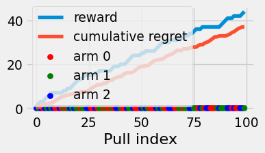
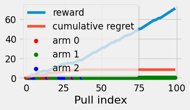
Theorem 4.1 (Pure exploration expected regret) The pure exploration strategy achieves regret $\Theta(T)$ in expectation.

Proof. By choosing arms uniformly at random,

\[ \mathop{\mathbb{E}}_{a_t\sim \text{Unif}([K])}[\mu^{a_t}] = \bar \mu := \frac{1}{K} \sum_{k=0}^{K-1} \mu^k \tag{4.8}\]

so the expected regret is simply

\[ \begin{aligned} \mathop{\mathbb{E}}[\text{Regret}_T] &= \sum_{t= 0}^{T-1} \mathop{\mathbb{E}}[\mu^\star - \mu^{a_t}] \\ &= T\cdot (\mu^\star - \bar \mu). \end{aligned} \tag{4.9}\]

This scales as $\Theta(T)$ in expectation, i.e. linear in the number of pulls $T$.

Code

agent = PureExploration(mab.K, mab.T)
mab_loop(mab, agent)
plot_strategy(mab, agent)

Figure 4.2: Reward and cumulative regret of the pure exploration algorithm.

Pure exploration doesn’t use any information about the environment to improve its strategy. The distribution over its arm choices always appears “(uniformly) random”.

4.4 Pure greedy

How might we improve on pure exploration? Instead, we could try each arm once, and then commit to the one with the highest observed reward. We’ll call this the pure greedy strategy.

Definition 4.5 (Pure greedy) On the $t$th pull, the arm $a_t$ is chosen according to

\[ a_t:= \begin{cases} t& t< K\\ \arg\max_{k\in [K]} r_k& t\ge K \end{cases} \tag{4.10}\]

where $r_t$ denotes the reward obtained on the $t$th pull.

Code

class PureGreedy(Agent):
    def choose_arm(self):
        """Choose the arm with the highest observed reward on its first pull."""
        return solutions.pure_greedy_choose_arm(self)

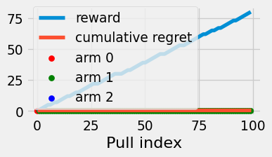
How does the expected regret of this strategy compare to that of pure exploration? We’ll do a more general analysis in the following section. Now, for intuition, suppose there’s just $K=2$ arms with means $\mu^1 > \mu^0$. If $r_1 > r_0$, then we repeatedly pull arm $1$ and achieve zero regret per pull. If $r_0 > r_1$, then we repeatedly pull arm $0$ and incur $\mu^1 - \mu^0$ regret per pull. Accounting for the first two pulls and the case of a tie, we obtain the following lower bound:

\[ \mathop{\mathbb{E}}[\text{Regret}_T] \ge \mathbb{P}(r^0 > r^1) T\cdot (\mu^1 - \mu^0) \tag{4.11}\]

This is still $\Theta(T)$, the same as pure exploration!

Code

agent = PureGreedy(mab.K, mab.T)
mab_loop(mab, agent)
plot_strategy(mab, agent)

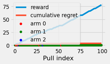
Figure 4.3: Reward and cumulative regret of the pure greedy algorithm.

The cumulative regret is a straight line because the regret only depends on the arms chosen and not the actual reward observed. In fact, we see in fig. 4.3 that the greedy algorithm can get lucky on the first set of pulls and act entirely optimally for that experiment! But its average regret is still linear, since the chance of sticking with a suboptimal arm is nonzero.

4.5 Explore-then-commit

We can improve the pure greedy algorithm (def. 4.5) as follows: let’s reduce the variance of the reward estimates by pulling each arm $N_\text{explore} \ge 1$ times before committing. This is called the explore-then-commit strategy.

Definition 4.6 (Explore-then-commit) The explore-then-commit algorithm first pulls each arm $N_\text{explore}$ times. Let

\[ \hat \mu^k:= \frac{1}{N_\text{explore}} \sum_{n=0}^{N_\text{explore}-1} r_{kN_\text{explore} + n} \tag{4.12}\]

denote the empirical mean reward of arm $k$ during these pulls. Afterwards, on the $t$th pull (for $t\ge N_\text{explore} K$), it chooses

\[ a_t:= \arg\max_{k\in [K]} \hat \mu^k. \tag{4.13}\]

Note that the “pure greedy” strategy above is just the special case where $N_\text{explore} = 1$.

Code

class ExploreThenCommit(Agent):
    def __init__(self, K: int, T: int, N_explore: int):
        super().__init__(K, T)
        self.N_explore = N_explore

    def choose_arm(self):
        return solutions.etc_choose_arm(self)

Code

agent = ExploreThenCommit(mab.K, mab.T, mab.T // 15)
mab_loop(mab, agent)
plot_strategy(mab, agent)

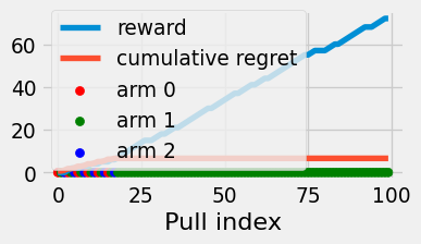
Figure 4.4: Reward and cumulative regret of the explore-then-commit algorithm

This algorithm finds the true optimal arm more frequently than the pure greedy strategy. We would expect ETC to then have a lower expected regret. We will show that ETC achieves the following regret bound:

Theorem 4.2 (ETC high-probability regret bound) The regret of ETC satisfies, with high probability,

\[ \text{Regret}_T= \widetilde{O}(T^{2/3} K^{1/3}), \tag{4.14}\]

where the tilde means we ignore logarithmic factors.

Proof. Let’s analyze the expected regret of the explore-then-commit strategy by splitting it up into the exploration and exploitation phases.

Exploration phase. This phase takes $N_\text{explore} K$ pulls. Since at each step we incur at most $1$ regret, the total regret is at most $N_\text{explore} K$.

Exploitation phase. This will take a bit more effort. We’ll prove that for any total time $T$, we can choose $N_\text{explore}$ such that with arbitrarily high probability, the regret is sublinear.

Let $\widehat{k}$ denote the arm chosen after the exploration phase. We know the regret from the exploitation phase is

\[ T_\text{exploit} (\mu^\star - \mu^{\widehat{k}}) \qquad \text{where} \qquad T_\text{exploit} := T- N_\text{explore} K. \tag{4.15}\]

So we’d need $\mu^\star - \mu^{\widehat{k}} \to 0$ as $T\to \infty$ in order to achieve sublinear regret. How can we do this?

Let’s define $\Delta^k:= \hat \mu^k- \mu^k$ to denote how far the mean estimate for arm $k$ is from the true mean. How can we bound this quantity? We’ll use the following useful inequality for i.i.d. bounded random variables:

Theorem 4.3 (Hoeffding’s inequality) Let $X_0, \dots, X_{N-1}$ be i.i.d. random variables with $X_n \in [0, 1]$ almost surely for each $n \in [N]$. Then for any $\delta > 0$,

\[ \mathbb{P}\left( \left| \frac{1}{N} \sum_{n=1}^N (X_n - \mathop{\mathbb{E}}[X_n]) \right| > \sqrt{\frac{\ln(2/\delta)}{2N}} \right) \le \delta. \tag{4.16}\]

Proof. The proof of this inequality is beyond the scope of this book. See Vershynin (2018, ch. 2.2).

We can apply this directly to the rewards for a given arm $k$, since the rewards from that arm are i.i.d.:

\[ \mathbb{P}\left(|\Delta^k| > \sqrt{ \frac{\ln(2/\delta)}{2N_\text{explore}} } \right) \le \delta. \tag{4.17}\]

This can be thought of as a $1-\delta$ confidence interval for the true arm mean $\mu^k$. But we can’t apply this to arm $\widehat{k}$ directly since $\widehat{k}$ is itself a random variable. Instead, we need to bound the error across all the arms simultaneously, so that the resulting bound will apply no matter what $\widehat{k}$ “crystallizes” to. The union bound provides a simple way to do this. (See Theorem A.1 for a review.)

In our case, we have one event per arm, stating that the CI for that arm contains the true mean. The probability that all of the CIs are accurate is then

\[ \begin{aligned} \mathbb{P}\left( \forall k\in [K] : |\Delta^k| \le \sqrt{\frac{\ln(2/\delta)}{2N_\text{explore}}} \right) &\ge 1- K\delta. \end{aligned} \tag{4.18}\]

This lower-bounds the probability that the CI for arm $\widehat{k}$ is accurate. Let us return to our original task of bounding $\mu^\star - \mu^{\widehat{k}}$. We apply the useful trick of “adding zero”:

\[ \begin{aligned} \mu^{k^\star} - \mu^{\widehat{k}} &= \mu^{k^\star} - \mu^{\widehat{k}} + (\hat \mu^{k^\star} - \hat \mu^{k^\star}) + (\hat \mu^{\widehat{k}} - \hat \mu^{\widehat{k}}) \\ &= \Delta^{\widehat{k}} - \Delta^{k^\star} + \underbrace{(\hat \mu^{k^\star} - \hat \mu^{\widehat{k}})}_{\le 0 \text{ by definition of } \widehat{k}} \\ &\le 2 \sqrt{\frac{\ln(2 K/ \delta')}{2N_\text{explore}}} \text{ with probability at least } 1-\delta' \end{aligned} \tag{4.19}\]

where we’ve set $\delta' := K\delta$. Putting this all together, we’ve shown that, with probability $1 - \delta'$,

\[ \text{Regret}_T\le N_\text{explore} K+ T_\text{exploit} \cdot \sqrt{\frac{2\ln(2 K/\delta')}{N_\text{explore}}}. \tag{4.20}\]

Note that it suffices for $N_\text{explore}$ to be on the order of $\sqrt{T}$ to achieve sublinear regret. In particular, we can find the optimal $N_\text{explore}$ by setting the derivative of eq. 4.20 with respect to $N_\text{explore}$ to zero:

\[ \begin{aligned} 0 &= K- T_\text{exploit} \cdot \frac{1}{2} \sqrt{\frac{2\ln(2 K/\delta')}{N_\text{explore}^3}} \\ N_\text{explore} &= \left( T_\text{exploit} \cdot \frac{\sqrt{\ln(2 K/ \delta')/2}}{ K} \right)^{2/3} \end{aligned} \tag{4.21}\]

Plugging this into the expression for the regret, we have (still with probability $1-\delta'$):

\[ \begin{aligned} \text{Regret}_T&\le 3 T^{2/3} \sqrt[3]{K\ln(2 K/\delta') / 2} \\ &= \widetilde{O}(T^{2/3} K^{1/3}), \end{aligned} \tag{4.22}\]

satisfying Theorem 4.2.

The ETC algorithm is rather “abrupt” in that it switches from exploration to exploitation after a fixed number of pulls. What if the total number of pulls $T$ isn’t known in advance? We’ll need to use a more gradual transition, which brings us to the epsilon-greedy algorithm.

4.6 Epsilon-greedy

Instead of doing all of the exploration and then all of the exploitation in separate phases, which requires knowing the time horizon beforehand, we can instead interleave exploration and exploitation by, at each pull, choosing a random action with some probability. We call this the epsilon-greedy algorithm.

Definition 4.7 (Epsilon-greedy) Let $N^k_t$ denote the number of times that arm $k$ is pulled within the first $t$ overall pulls, and let $\hat \mu^k_t$ denote the sample mean of the corresponding rewards:

\[ \begin{aligned} N^k_t&:= \sum_{t' = 0}^{t-1} \mathbf{1} \{ a_{t'} = k\}, \\ \hat \mu^k_t&:= \frac{1}{N^k_t} \sum_{t' = 0}^{t-1} \mathbf{1} \{ a_{t'} = k\} r_{t'}. \\ \end{aligned} \tag{4.23}\]

On the $t$th pull, the arm $a_t$ is chosen according to

\[ a_t:= \begin{cases} \text{sample from } \text{Unif}([K]) & \text{with probability } \epsilon_t\\ \arg\max_{k\in [K]} \hat \mu^k_t& \text{with probability } 1 - \epsilon_t, \end{cases} \tag{4.24}\]

where $\epsilon_t\in [0, 1]$ is the probability of choosing a random action.

Code

class EpsilonGreedy(Agent):
    def __init__(
        self,
        K: int,
        T: int,
        ε_array: Float[Array, " T"],
    ):
        super().__init__(K, T)
        self.ε_array = ε_array

    def choose_arm(self):
        return solutions.epsilon_greedy_choose_arm(self)

Code

agent = EpsilonGreedy(mab.K, mab.T, np.full(mab.T, 0.1))
mab_loop(mab, agent)
plot_strategy(mab, agent)

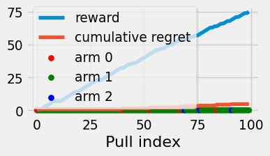
Figure 4.5: Reward and cumulative regret of the epsilon-greedy algorithm

We let the exploration probability $\epsilon_t$ vary over time. This lets us gradually decrease $\epsilon_t$ as we learn more about the reward distributions and no longer need to explore as much.

Exercise 4.2 (Regret for constant epsilon) What is the asymptotic expected regret of the algorithm if we set $\epsilon$ to be a constant? Is this different from pure exploration (def. 4.4)?

Theorem 4.4 (Epsilon-greedy expected regret) Let $\epsilon_t:= \sqrt[3]{K\ln(t) / t}$. Then the epsilon-greedy achieves a regret of $\widetilde O(t^{2/3} K^{1/3})$ in expectation (ignoring logarithmic factors).

Proof. We won’t prove this here. See Agarwal et al. (2022) for a proof.

In ETC, we had to set $N_\text{explore}$ based on the total number of pulls $T$. But the epsilon-greedy algorithm handles the exploration incrementally: the regret rate holds for any $t$, and doesn’t depend on the total number of pulls $T$.

But the way epsilon-greedy and ETC explore is rather naive: they explore uniformly across all the arms. But what if we could be smarter about it, and explore more for arms that we’re less certain about?

4.7 Upper Confidence Bound (UCB)

The upper confidence bound algorithm is the first strategy we study that explores adaptively: it identifies arms it is less certain about, and explicitly trades off between learning more about these and exploiting arms that already seem good.

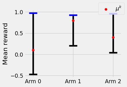
To quantify how certain we are about the mean of each arm, UCB computes statistical confidence intervals (CIs) for the arm means, and then chooses the arm with the highest upper confidence bound (hence its name). Concretely, after $t$ pulls, we compute upper confidence bounds $M^k_t$ for each arm $k$ such that $\mu^k\le M^k_t$ with high probability, and select $a_t:= \arg \max_{k\in [K]} M^k_t$. This operates on the principle of the benefit of the doubt (i.e. optimism in the face of uncertainty): we’ll choose the arm that we’re most optimistic about.

Code

means = [0.1, 0.8, 0.4]
lower_bounds = [-0.4745434, 0.2002283, 0.04175852]
upper_bounds = [0.9745434, 0.9247717, 0.95824148]

whiskers = np.array([lower_bounds, upper_bounds])

fig, ax = plt.subplots()
for i in range(len(means)):
    ax.plot([i, i], [whiskers[0, i], whiskers[1, i]], color='black')
    ax.plot([i - 0.1, i + 0.1], [whiskers[0, i], whiskers[0, i]], color='black')
    ax.plot([i - 0.1, i + 0.1], [whiskers[1, i], whiskers[1, i]], color='blue')

ax.scatter(range(len(means)), means, color='red', zorder=5, label="$\mu^k$")
ax.set_xticks(range(len(means)))
ax.set_xticklabels([f'Arm {i}' for i in range(3)])
ax.set_ylabel(r'Mean reward')
fig.legend()
plt.show()

Figure 4.6: Visualization of confidence intervals for the arm means. UCB would choose arm $0$ since it has the highest upper confidence bound.

Theorem 4.5 (Confidence intervals for arm means) As in our definition of the epsilon-greedy algorithm (def. 4.7), let $N^k_t$ denote the number of times we pull arm $k$ within the first $t$ pulls, and let $\hat \mu^k_t$ denote the sample mean of the corresponding rewards. Then with probability at least $1 - \delta$, for all $t\ge K$,

\[ \mu^k\in \left[ \hat \mu^k_t- \frac{1}{\sqrt{N^k_t}} \cdot \sqrt{ \frac{\ln(2 t/\delta)}{2} }, \hat \mu^k_t+ \frac{1}{\sqrt{N^k_t}} \cdot \sqrt{ \frac{\ln(2 t/\delta)}{2} } \right]. \tag{4.25}\]

We assume that during the first $K$ pulls, we pull each arm once.

Definition 4.8 (Upper confidence bound algorithm (Auer, 2002)) The UCB algorithm first pulls each arm once. Then it chooses the $t$th pull (for $t\ge K$) by taking

\[ a_t:= \arg\max_{k\in [K]} \hat \mu^k_t+ \sqrt{ \frac{\ln(2 t/\delta)}{2 N^k_t} }, \tag{4.26}\]

where $\delta \in (0, 1)$ is a parameter that controls the width of the confidence interval.

Intuitively, UCB prioritizes arms where:

$\hat \mu^k_t$ is large, i.e. the arm’s corresponding sample mean is high, and we’d choose it for exploitation, and
$\sqrt{\frac{\ln(2 t/\delta)}{2N^k_t}}$ is large, i.e. $N^k_t$ is small and we’re still uncertain about the arm, and we’d choose it for exploration.

$\delta$ is formally the coverage probability of the confidence interval, but we can also treat it as a parameter that trades off between exploration and exploitation:

A smaller $\delta$ would give us a larger interval, emphasizing the exploration term.
A larger $\delta$ would give a tighter interval, prioritizing the current sample means.

We now prove Theorem 4.5.

Proof. Our proof is similar to that in Theorem 4.2: we use Hoeffding’s inequality to construct a CI for the mean of a bounded random variable (i.e. the rewards from a given arm). However, we must be careful, since the number of samples from arm $k$ up to time $t$, $N^k_t$, is a random variable.

Hoeffding’s inequality (Theorem 4.3) tells us that, for $N$ i.i.d. samples $\widetilde r_0, \dots, \widetilde r_{N-1}$ from arm $k$,

\[ | \widetilde \mu^k_N - \mu^k| \le \sqrt{ \frac{\ln( 2 / \delta )}{2 N} } \tag{4.27}\]

with probability at least $1 - \delta$, where $\widetilde \mu^k_N = \frac{1}{N} \sum_{n=0}^{N-1} \widetilde r_n$. The union bound then tells us that with probability at least $1 - \delta'$, for all $N = 1, \dots, t$,

\[ \forall N = 1, \dots, t: | \widetilde \mu^k_N - \mu^k| \le \sqrt{ \frac{\ln( 2 t/ \delta' )}{2 N} }. \tag{4.28}\]

Since $N^k_t\in \{ 1, \dots, t\}$ (we assume each arm is pulled once at the start), eq. 4.28 implies that

\[ | \widetilde \mu^k_{N^k_t} - \mu^k| \le \sqrt{ \frac{\ln( 2 t/ \delta' )}{N} } \tag{4.29}\]

with probability at least $1 - \delta'$ as well. But notice that $\widetilde \mu^k_{N^k_t}$ is identically distributed to $\hat \mu^k_t$: both refer to the sample mean of the first $N^k_t$ pulls from arm $k$. This gives the bound in Theorem 4.5 (after relabelling $\delta' \mapsto \delta$).

Code

class UCB(Agent):
    def __init__(self, K: int, T: int, delta: float):
        super().__init__(K, T)
        self.delta = delta

    def choose_arm(self):
        return solutions.ucb_choose_arm(self)

Code

agent = UCB(mab.K, mab.T, 0.9)
mab_loop(mab, agent)
plot_strategy(mab, agent)

Figure 4.7: Reward and cumulative regret of the upper confidence bound algorithm

As desired, this explores in a smarter, adaptive way compared to the previous algorithms. Does it achieve lower regret?

Theorem 4.6 (UCB high-probability regret bound) With probability $1-\delta''$,

\[ \text{Regret}_T= \widetilde O(K\sqrt{T}) \tag{4.30}\]

Proof. First we’ll bound the regret incurred at each timestep. Then we’ll bound the total regret across timesteps.

For the sake of analysis, we’ll use a slightly looser bound that applies across the whole time horizon and across all arms. We’ll omit the derivation since it’s very similar to the above (walk through it yourself for practice).

\[ \begin{aligned} \mathbb{P}\left(\forall k\le K, t< T: |\hat \mu^k_t- \mu^k| \le B^k_t\right) &\ge 1-\delta'' \\ \text{where} \quad B^k_t&:= \sqrt{\frac{\ln(2 TK/\delta'')}{2 N^k_t}}. \end{aligned} \tag{4.31}\]

Intuitively, $B^k_t$ denotes the width of the CI for arm $k$ at time $t$. Then, assuming the above uniform bound holds (which occurs with probability $1-\delta''$), we can bound the regret at each timestep as follows:

\[ \begin{aligned} \mu^\star - \mu^{a_t} &\le \hat \mu^{k^\star}_t+ B_t^{k^\star} - \mu^{a_t} && \text{applying UCB to arm } k^\star \\ &\le \hat \mu^{a_t}_t+ B^{a_t}_t- \mu^{a_t} && \text{since UCB chooses } a_t= \arg \max_{k\in [K]} \hat \mu^k_t+ B_t^{k} \\ &\le 2 B^{a_t}_t&& \text{since } \hat \mu^{a_t}_t- \mu^{a_t} \le B^{a_t}_t\text{ by definition of } B^{a_t}_t\\ \end{aligned} \tag{4.32}\]

Summing this across timesteps gives

\[ \begin{aligned} \text{Regret}_T&\le \sum_{t= 0}^{T-1} 2 B^{a_t}_t\\ &= \sqrt{2\ln(2 TK/\delta'')} \sum_{t= 0}^{T-1} (N^{a_t}_t)^{-1/2} \\ \sum_{t= 0}^{T-1} (N^{a_t}_t)^{-1/2} &= \sum_{t= 0}^{T-1} \sum_{k=0}^{K-1} \mathbf{1}\{ a_t= k \} (N^k_t)^{-1/2} \\ &= \sum_{k=0}^{K-1} \sum_{n=1}^{N_T^k} n^{-1/2} \\ &\le K \sum_{n=1}^Tn^{-1/2} \\ \sum_{n=1}^Tn^{-1/2} &\le 1 + \int_1^Tx^{-1/2} \ \mathrm{d}x \\ &= 1 + (2 \sqrt{x})_1^T\\ &= 2 \sqrt{T} - 1 \\ &\le 2 \sqrt{T} \\ \end{aligned} \]

Putting everything together gives, with probability $1-\delta''$,

\[ \begin{aligned} \text{Regret}_T&\le 2 K\sqrt{2 T\ln(2 TK/\delta'')} \\ &= \widetilde O(K\sqrt{T}), \end{aligned} \tag{4.33}\]

as in Theorem 4.6.

In fact, we can do a more sophisticated analysis to trim off a factor of $\sqrt{K}$ and show $\text{Regret}_T= \widetilde O(\sqrt{TK})$.

4.7.1 Lower bound on regret (intuition)

Is it possible to do better than $\Omega(\sqrt{T})$ in general? In fact, no! We can show that any algorithm must incur $\Omega(\sqrt{T})$ regret in the worst case. We won’t rigorously prove this here, but the intuition is as follows.

The Central Limit Theorem tells us that with $T$ i.i.d. samples from some distribution, we can only learn the mean of the distribution to within $\Omega(1/\sqrt{T})$ (the standard deviation). Then, since we get $T$ samples spread out across the arms, we can only learn each arm’s mean to an even looser degree.

That is, if two arms have means that are within about $1/\sqrt{T}$, we won’t be able to confidently tell them apart, and will sample them about equally. But then we’ll incur regret \[ \Omega((T/2) \cdot (1/\sqrt{T})) = \Omega(\sqrt{T}). \tag{4.34}\]

4.8 Thompson sampling and Bayesian bandits

So far, we’ve treated the parameters $\mu^0, \dots, \mu^{K-1}$ of the reward distributions as fixed. Instead, we can take a Bayesian approach where we treat them as random variables from some prior distribution. Then, upon pulling an arm and observing a reward, we can simply condition on this observation to exactly describe the posterior distribution over the parameters. This fully describes the information we gain about the parameters from observing the reward.

From this Bayesian perspective, the Thompson sampling algorithm follows naturally: just sample from the distribution of the optimal arm, given the observations!

Code

class Distribution:
    def sample(self) -> Float[Array, " K"]:
        """Sample a vector of means for the K arms."""
        ...

    def update(self, arm: int, reward: float):
        """Condition on obtaining `reward` from the given arm."""
        ...

Code

class ThompsonSampling(Agent):
    def __init__(self, K: int, T: int, prior: Distribution):
        super().__init__(K, T)
        self.distribution = prior

    def choose_arm(self):
        means = self.distribution.sample()
        return random_argmax(means)

    def update_history(self, arm: int, reward: int):
        super().update_history(arm, reward)
        self.distribution.update(arm, reward)

In other words, we sample each arm proportionally to how likely we think it is to be optimal, given the observations so far. This strikes a good exploration-exploitation tradeoff: we explore more for arms that we’re less certain about, and exploit more for arms that we’re more certain about. Thompson sampling is a simple yet powerful algorithm that achieves state-of-the-art performance in many settings.

Example 4.4 (Bayesian Bernoulli bandit) We’ve been working in the Bernoulli bandit setting, where arm $k$ yields a reward of $1$ with probability $\mu^k$ and no reward otherwise. The vector of success probabilities $\boldsymbol{\mu} = (\mu^0, \dots, \mu^{K-1})$ thus describes the entire MAB.

Under the Bayesian perspective, we think of $\boldsymbol{\mu}$ as a random vector drawn from some prior distribution $p \in \triangle([0, 1]^K)$. For example, we might have $p$ be the Uniform distribution over the unit hypercube $[0, 1]^K$, that is,

\[ p(\boldsymbol{\mu}) = \begin{cases} 1 & \text{if } \boldsymbol{\mu}\in [0, 1]^K\\ 0 & \text{otherwise} \end{cases} \tag{4.35}\]

In this case, upon viewing some reward, we can exactly calculate the posterior distribution of $\boldsymbol{\mu}$ using Bayes’s rule (i.e. the definition of conditional probability):

\[ \begin{aligned} \mathbb{P}(\boldsymbol{\mu} \mid a_0, r_0) &\propto \mathbb{P}(r_0 \mid a_0, \boldsymbol{\mu}) \mathbb{P}(a_0 \mid \boldsymbol{\mu}) \mathbb{P}(\boldsymbol{\mu}) \\ &\propto (\mu^{a_0})^{r_0} (1 - \mu^{a_0})^{1-r_0}. \end{aligned} \]

This is the PDF of the $\text{Beta}(1 + r_0, 1 + (1 - r_0))$ distribution, which is a conjugate prior for the Bernoulli distribution. That is, if we start with a Beta prior on $\mu^k$ (note that $\text{Unif}([0, 1]) = \text{Beta}(1, 1)$), then the posterior, after conditioning on samples from $\text{Bern}(\mu^k)$, will also be Beta. This is a very convenient property, since it means we can simply update the parameters of the Beta distribution upon observing a reward, rather than having to recompute the entire posterior distribution from scratch.

Code

class Beta(Distribution):
    def __init__(self, K: int, alpha: int = 1, beta: int = 1):
        self.alphas = np.full(K, alpha)
        self.betas = np.full(K, beta)

    def sample(self):
        return np.random.beta(self.alphas, self.betas)

    def update(self, arm: int, reward: int):
        self.alphas[arm] += reward
        self.betas[arm] += 1 - reward

Code

beta_distribution = Beta(mab.K)
agent = ThompsonSampling(mab.K, mab.T, beta_distribution)
mab_loop(mab, agent)
plot_strategy(mab, agent)

Figure 4.8: Reward and cumulative regret of the Thompson sampling algorithm

It turns out that asymptotically, Thompson sampling is optimal in the following sense. Lai & Robbins (1985) prove an instance-dependent lower bound that says for any bandit algorithm,

\[ \liminf_{T\to \infty} \frac{\mathop{\mathbb{E}}[N_T^k]}{\ln(T)} \ge \frac{1}{\mathrm{KL}\left(\mu^k\parallel\mu^\star\right)} \tag{4.36}\]

where

\[ \mathrm{KL}\left(\mu^k\parallel\mu^\star\right) := \mu^k\ln \frac{\mu^k}{\mu^\star} + (1 - \mu^k) \ln \frac{1 - \mu^k}{1 - \mu^\star} \tag{4.37}\]

measures the Kullback-Leibler divergence from the Bernoulli distribution with mean $\mu^k$ to the Bernoulli distribution with mean $\mu^\star$. It turns out that Thompson sampling achieves this lower bound with equality! That is, not only is the error rate optimal, but the constant factor is optimal as well.

4.9 Contextual bandits

In the multi-armed bandits setting described above, each pull is exactly the same. We don’t obtain any prior information about the reward distributions. However, consider the online advertising example (ex. 4.1), where each arm corresponds to an ad we could show a given user, and we receive a reward if and only if the user clicks on the ad. Suppose Alice is interested in sports and politics, while Bob is interested in news and entertainment. The ads that Alice is likely to click differ from those that Bob is likely to click. That is, the reward distributions of the arms depend on some prior context. We can model such environments using contextual bandits.

Definition 4.9 (Contextual bandit) At each pull $t$, a context $x_t$ is chosen from the set $\mathcal{X}$ of all possible contexts. The learner gets to observe the context before they choose an action. That is, we treat the action chosen on the $t$th pull as a function of the context: $a_t(x_t)$. Then, the learner observes the reward from the chosen arm, where the reward distribution also depends on the context.

Example 4.5 (Online advertising as a contextual bandit problem) Suppose you represent an online advertising company and you are tasked with placing ads on the New York Times website. Articles are categorized into six sections, each with its own web page: U.S., World, Business, Arts, Lifestyle, and Opinion. You might decide to frame this as a contextual bandits problem with $|\mathcal{X}| = 6$. This is because the demographic of readers likely differs across the different pages, and so the reward distributions differ across pages accordingly.

Suppose our context is discrete, as in ex. 4.5. Then we could treat each context as its own MAB, assigning each context-arm pair to a distinct arm in an enlarged MAB of $K|\mathcal{X}|$ arms.

Exercise 4.3 (Naive UCB for contextual bandits) Write down the UCB algorithm for this enlarged MAB. That is, write an expression $M^k_t$ in terms of $K$ and $|\mathcal{X}|$ such that $a_t(x_t) = \arg\max_{k\in [K]} M^k_t$.

Recall that executing UCB for $T$ timesteps on an MAB with $K$ arms achieves a regret bound of $\widetilde{O}(\sqrt{TK})$ (Theorem 4.6). So in this problem, we would achieve regret $\widetilde{O}(\sqrt{TK|\mathcal{X}|})$ in the contextual MAB, which has a polynomial dependence on $|\mathcal{X}|$. But in a situation where we have too many possible contexts, or the context is a continuous value, this algorithm no longer works.

Note that this “enlarged MAB” treats the different contexts as entirely unrelated to each other, while in practice, often contexts are related to each other in some way. In the medical trial example (ex. 4.2), clients with similar health situations may benefit from the same medications. How can we incorporate this structure into our solution?

4.9.1 Linear contextual bandits

Remark 4.5 (Supervised learning). The material in this section depends on basic knowledge of supervised learning (Chapter 5).

Suppose now that we observe a vector-valued context, that is, $\mathcal{X} = \mathbb{R}^D$. For example, in a medical trial (ex. 4.2), we might know the patient’s height, age, blood pressure, etc., each of which would be a separate element of the vector. The approach of treating each context as its own MAB problem no longer works out-of-the-box since the number of contexts is infinite. Instead, we assume that the mean reward of each arm $k$ is a function of the context: $\mu^k: \mathcal{X} \to \mathbb{R}$.

Rather than the Bernoulli bandit problem (def. 4.1), we’ll assume that the mean reward is linear in the context. (This model is easier to work with for our purposes.) That is, a reward $r^k$ from arm $k$ is drawn according to

\[ r^k= x^\top \theta^k+ \varepsilon, \tag{4.38}\]

where $\theta^k\in \mathbb{R}^D$ describes a feature direction for arm $k$ and $\varepsilon$ is some independent noise with mean $0$ and variance $\sigma^2$. This clearly has

\[ \mu^k(x) = x^\top \theta^k. \tag{4.39}\]

Then, on the $t$th pull, given context $x_t$, we can model the mean reward from arm $k$ as

\[ \hat \mu^k_t(x_t) := x_t^\top \hat \theta^k_t, \tag{4.40}\]

where $\hat \theta^k_t$ is some estimator of $\theta^k$ computed from the first $t$ pulls.

Remark 4.6 (Assumptions for linear models). Why did we switch from Bernoulli reward distributions to the additive model in eq. 4.38? The estimator eq. 4.40 is a bit odd for the Bernoulli bandit problem: since $\mu^k$ is the success probability of arm $k$, it would have to lie between $0$ and $1$, but $\hat \mu^k_t(x_t)$ extends outside this interval. The question of how to model the unknown parameters of a distribution is a supervised learning problem (Chapter 5). For instance, in Bernoulli bandit, we could instead use a logistic regression model for each arm’s success probability. We won’t dive into more advanced supervised learning topics here.

Our goal is still to develop an algorithm that chooses an arm $a_t(x_t)$ to pull based on the experience gained during the first $t$ trials. We will use supervised learning, in particular, empirical risk minimization (Section 5.3), to estimate $\theta^k$ for each arm. That is, we compute $\hat \theta^k_t$ as the vector that minimizes squared error from the observed rewards:

\[ \hat \theta_t^k:= \arg\min_{\theta \in \mathbb{R}^D} \sum_{t' \in \mathcal{I}^k_t} (r_{t'} - x_{t'}^\top \theta)^2, \tag{4.41}\]

where

\[ \mathcal{I}^k_t:= \{ t' \in [t] \mid a_{t'} = k\} \tag{4.42}\]

denotes the subset of $[t]$ at which arm $k$ was pulled. Note that $|\mathcal{I}^k_t| = N^k_t$ as defined in eq. 4.23. The ERM problem in eq. 4.41 has the closed-form solution known as the ordinary least squares (OLS) estimator:

\[ \begin{aligned} \hat \theta_t^k&= (\widehat \Sigma_t^k)^{-1}\left( \frac{1}{N^k_t} \sum_{t' \in \mathcal{I}^k_t} x_{t'} r_{t'} \right) \\ \text{where} \quad \widehat \Sigma_t^k&= \frac{1}{N^k_t} \sum_{t' \in \mathcal{I}^k_t} x_{t'} x_{t'}^\top. \end{aligned} \tag{4.43}\]

$\widehat \Sigma_t^k$ is the (biased) empirical covariance matrix of the contexts across the trials where arm $k$ was pulled (out of the first $t$ trials).

Remark 4.7 (Invertibility). In eq. 4.43, we write the expression $(\widehat \Sigma_t^k)^{-1}$, assuming that $\widehat \Sigma_t^k$ is invertible. This only holds if the context features are linearly independent, that is, there does not exist some coordinate $d \in [D]$ that can be written as a linear combination of the other coordinates. One way to ensure that $\widehat \Sigma_t^k$ is invertible is to add a $\lambda I$ regularization term to it. This is equivalent to solving a ridge regression problem instead of the unregularized least squares problem.

Now, given a sequence of $t$ contexts, pulls, and rewards $x_0, a_0, r_0, \dots, x_{t-1}, a_{t-1}, r_{t-1}$, we can estimate $\mu^k(x_t)$ for each arm. This is helpful, but we haven’t yet solved the problem of deciding which arms to pull in each context to trade off between exploration and exploitation.

The upper confidence bound (UCB) algorithm (def. 4.8) was a useful strategy. What would we need to adapt UCB to this new setting? Recall that at each step, UCB estimates a confidence interval for each arm mean, and chooses the arm with the highest upper confidence bound. We already have an estimator $\hat \mu^k_t(x_t)$ of each arm mean, so all that is left is to compute the width of the confidence interval itself.

Theorem 4.7 (LinUCB confidence interval) Suppose we pull each arm once during the first $K$ trials. Then at each pull $t\ge K$, for all arms $k\in [K]$ and all contexts $x \in \mathcal{X}$, we have that with probability at least $1 - 1/\beta^2$,

\[ \mu^k(x) \in \left[ x^\top \hat \theta^k_t - \beta \frac{\sigma}{\sqrt{N^k_t}} \cdot \sqrt{x^\top (\widehat \Sigma^k_t)^{-1} x}, x^\top \hat \theta^k_t + \beta \frac{\sigma}{\sqrt{N^k_t}} \cdot \sqrt{x^\top (\widehat \Sigma^k_t)^{-1} x} \right], \tag{4.44}\]

where

$\sigma$ is the standard deviation of the reward (eq. 4.38),
$N^k_t$ is the number of times arm $k$ was pulled in the first $t$ pulls (eq. 4.23),
$\hat \theta^k_t$ is the OLS estimator for arm $k$ (eq. 4.43),
and $\widehat \Sigma^k_t$ is the sample covariance matrix of the contexts given arm $k$ (eq. 4.43).

We can then plug this interval into the UCB strategy (def. 4.8) to obtain what is known as the LinUCB algorithm:

Definition 4.10 (LinUCB (Li et al., 2010)) LinUCB first pulls each arm once. Then, for pull $t\ge K$, LinUCB chooses an arm according to

\[ a_t(x_t) := \arg\max_{k\in [K]} x^\top \hat \theta^k_t + \beta \frac{\sigma}{\sqrt{N^k_t}} \sqrt{x_t^\top (\widehat \Sigma^k_t)^{-1} x_t}, \tag{4.45}\]

where $\sigma, N^k_t, \hat \theta^k_t, \widehat \Sigma^k_t$ are defined as in Theorem 4.7, and $\beta > 0$ controls the width of the confidence interval (and thereby the exploration-exploitation tradeoff).

The first term is exactly our predicted mean reward $\hat \mu^k_t(x_t)$. We can think of it as the term encouraging exploitation of an arm if its predicted mean reward is high. The second term is the width of the confidence interval given by Theorem 4.7. This is the exploration term that encourages an arm when $x_t$ is not aligned with the data seen so far, or if arm $k$ has not been explored much and so $N_t^k$ is small.

Now we prove Theorem 4.7.

Proof. How can we construct the upper confidence bound in Theorem 4.7? Previously, we treated the pulls of an arm as i.i.d. samples and used Hoeffding’s inequality to bound the distance of the sample mean, our estimator, from the true mean. However, now our estimator is not a sample mean, but rather the OLS estimator above eq. 4.43. We will construct the confidence interval using Chebyshev’s inequality, which gives a confidence interval for the mean of a distribution based on that distribution’s variance.

Theorem 4.8 (Chebyshev’s inequality) For a random variable $Y$ with mean $\mu$ and variance $\sigma^2$,

\[ |Y - \mu| \le \beta \sigma \quad \text{with probability} \ge 1 - \frac{1}{\beta^2} \tag{4.46}\]

We want to construct a CI for $x^\top \theta^k$, the mean reward from arm $k$. Our estimator is $x^\top \hat \theta^k_t$. Applying Chebyshev’s inequality requires us to compute the variance of our estimator.

Theorem 4.9 (Variance of OLS) Given the linear reward model in eq. 4.38,

\[ \text{Var}(x^\top \hat \theta_t^k) = \frac{\sigma^2}{N^k_t} x^\top (\widehat \Sigma^t_k)^{-1} x, \tag{4.47}\]

where $\widehat \Sigma^t_k$ is defined in eq. 4.43.

Proof. We leave the proof as an exercise. It follows from applications of the law of iterated expectations.

Now we can substitute eq. 4.47 into eq. 4.46 to obtain the desired CI:

\[ \begin{aligned} x_t^\top \theta^k\le x_t^\top \hat \theta_t^k + \beta \sqrt{x_t^\top (A_t^k)^{-1} x_t} \quad \text{with probability} \ge 1 - \frac{1}{\beta^2} \end{aligned} \tag{4.48}\]

Code

class LinUCBPseudocode(Agent):
    def __init__(
        self, K: int, T: int, D: int, lam: float, get_c: Callable[[int], float]
    ):
        super().__init__(K, T)
        self.lam = lam
        self.get_c = get_c
        self.contexts = [None for _ in range(K)]
        self.A = np.repeat(lam * np.eye(D)[...], K)  # regularization
        self.targets = np.zeros(K, D)
        self.w = np.zeros(K, D)

    def choose_arm(self, context: Float[Array, " D"]):
        c = self.get_c(self.count)
        scores = self.w @ context + c * np.sqrt(
            context.T @ np.linalg.solve(self.A, context)
        )
        return random_argmax(scores)

    def update_history(self, context: Float[Array, " D"], arm: int, reward: int):
        self.A[arm] += np.outer(context, context)
        self.targets[arm] += context * reward
        self.w[arm] = np.linalg.solve(self.A[arm], self.targets[arm])

4.10 Key takeaways

In this chapter, we explored the multi-armed bandit setting for analyzing sequential decision-making in an unknown environment. An MAB consists of multiple arms, each with an unknown reward distribution. The agent’s task is to learn about these through interaction, eventually minimizing the regret, which measures how suboptimal the chosen arms were.

We saw algorithms such as upper confidence bound and Thompson sampling that handle the tradeoff between exploration and exploitation, that is, the tradeoff between choosing arms that the agent is uncertain about and arms the agent already supposes are be good.

We finally discussed contextual bandits, in which the agent gets to observe some context that affects the reward distributions. We can approach these problems through supervised learning approaches.

4.11 Bibliographic notes and further reading

The problem that a bandit algorithm faces after $t$ pulls is to infer differences between the means of a set of distributions given $t$ samples spread out across those distributions. This is a well-studied problem in statistics.

A common practice in various fields such as psychology is to compare within-group variances to the variance of the group means. This popular class of methods is known as analysis of variance (ANOVA). It has been studied at least since Laplace in the 1770s (Stigler, 2003) and was further popularized by Fisher (1925). William Thompson studied the two-armed mean distinction problem in Thompson (1933) and Thompson (1935). Our focus has been on the decision-making aspect of the bandit problem, rather than the hypothesis testing aspect.

Adding the sequential decision-making aspect turns the above into the full multi-armed bandit problem. Wald (1949) studies the sequential analysis problem in depth. Robbins (1952) then builds on Wald’s work and provides a clear exposition of the bandit problem in the form presented in this chapter. Berry & Fristedt (1985) is a comprehensive treatment of bandit problems from a statistical perspective.

Remark 4.8 (Disambiguation of LinUCB). The name “LinUCB” is used for various similar algorithms throughout the literature. Here we use it as defined in Li et al. (2010). This algorithm was also considered in Auer (2002), the paper that introduced UCB, under the name “Associative Reinforcement Learning with Linear Value Functions”.