Code
import numpy as np
import matplotlib.pyplot as plt
from utils import latex
import numpy as np
import matplotlib.pyplot as plt
import controlIn Chapter 2, we considered decision problems with finitely many states and actions. However, in many applications, states and actions may take on continuous values. For example, consider autonomous driving, controlling a robot’s joints, and automated manufacturing. How can we teach computers to solve these kinds of problems? This is the task of continuous control.
Aside from the change in the state and action spaces, the general problem setup remains the same: we seek to construct an optimal policy that outputs actions to solve the desired task. We will see that many key ideas and algorithms, in particular dynamic programming algorithms (Section 2.3.2), carry over to this new setting.
This chapter introduces a fundamental tool to solve a simple class of continuous control problems: the linear quadratic regulator (LQR). We can use the LQR model as a building block for solving more complex problems.
Remark 3.1 (Control vs RL). Control theory is often considered a distinct, though related, field from RL. In both fields, the central aim is to solve sequential decision problems, i.e. find a strategy for taking actions in the environment in order to achieve some goal that is measured by a scalar signal. The two fields arose rather independently and with rather different problem settings, and use different mathematical terminology as a result.
Control theory has close ties to electrical and mechanical engineering. Control theorists typically work in a continuous-time setting in which the dynamics can be described by systems of differential equations. The goal is typically to ensure stability of the system and minimize some notion of “cost” (e.g. wasted energy in controlling the system). Rather than learning the system from data, one typically supposes a particular structure of the environment and solves for the optimal controller using analytical or numerical methods. As such, most control theory algorithms, like the ones we will explore in this chapter, are planning methods that do not require learning from data.
import numpy as np
import matplotlib.pyplot as plt
from utils import latex
import numpy as np
import matplotlib.pyplot as plt
import controlLet’s first look at a simple example of a continuous control problem:
Example 3.1 (CartPole) Try to balance a pencil on its point on a flat surface. It’s much more difficult than it may first seem: the position of the pencil varies continuously, and the state transitions governing the system, i.e. the laws of physics, are highly complex. This task is equivalent to the classic control problem known as CartPole:
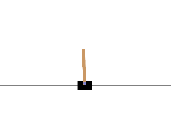
The state \(x\in \mathbb{R}^4\) can be described by four real variables:
We can control the cart by applying a horizontal force \(u\in \mathbb{R}\).
Goal: Stabilize the cart around an ideal state and action \((x^\star, u^\star)\).
A continuous control environment is a special case of an MDP (def. 2.4). Recall that a finite-horizon MDP
\[ \mathcal{M} = (\mathcal{S}, \mathcal{A}, P_0, P, r, H). \tag{3.1}\]
is defined by its state space \(\mathcal{S}\), action space \(\mathcal{A}\), initial state distribution \(P_0\), state transitions \(P\), reward function \(r\), and time horizon \(H\). These each have equivalents in the control setting.
Definition 3.1 (Continuous control environment) A continuous control environment is defined by the following components:
Together, these constitute a description of the environment
\[ \mathcal{M} = (\mathcal{S}, \mathcal{A}, P_0, f, \nu, c, H). \tag{3.3}\]
Definition 3.2 (Optimal control) For a continuous control environment \(\mathcal{M}\), the optimal control problem is to compute a policy \(\pi\) that minimizes the total cost
\[ \begin{aligned} \min_{\pi_0, \dots, \pi_{H-1} : \mathcal{S} \to \mathcal{A}} \quad & \mathop{\mathbb{E}}\left[ \sum_{h=0}^{H-1} c_h(x_h, u_h) \right] \\ \text{where} \quad & x_{h+1} = f_h(x_h, u_h, w_h), \\ & u_h= \pi_h(x_h) \\ & x_0 \sim P_0 \\ & w_h\sim \nu_h. \end{aligned} \tag{3.4}\]
In this chapter, we will only consider deterministic, time-dependent policies
\[ \pi = (\pi_0, \dots, \pi_{H-1}) \quad \text{where} \quad \pi_h : \mathcal{S} \to \mathcal{A} \text{ for each } h\in [H]. \tag{3.5}\]
To make the explicit conditioning more concise, we let \(\rho^\pi\) denote the trajectory distribution induced by the policy \(\pi\). That is, if we sample initial states from \(P_0\), act according to \(\pi\), and transition according to the dynamics \(f\), the resulting distribution over trajectories is \(\rho^\pi\). Put another way, the procedure for sampling from \(\rho^\pi\) is to take rollouts in the environment using \(\pi\).
Theorem 3.1 (Trajectory distributions) Let \(\pi = \{ \pi_0, \dots, \pi_{H-1} \}\) be a deterministic, time-dependent policy. We include states \(x_h\), actions \(u_h\), and noise terms \(w_h\) in the trajectory. Then the density of a trajectory \(\tau = (x_0, u_0, w_0, \dots, w_{H-2}, x_{H-1}, u_{H-1})\) can be expressed as follows:
\[ \begin{aligned} \rho^{\pi}(\tau) &:= P_0(x_0) \times \mathbf{1}\left\{u_0 = \pi_0(x_0)\right\} \\ &\quad {} \times \nu(w_0) \times \mathbf{1}\left\{x_1 = f(x_0, u_0, w_0)\right\} \\ &\quad {} \times \cdots \\ &\quad {} \times \nu(w_{H-2}) \times \mathbf{1}\left\{x_{H-1} = f(x_{H-2}, u_{H-2}, w_{H-2})\right\} \times \mathbf{1}\left\{u_{H-1} = \pi_{H-1}(x_{H-1})\right\} \\ &= P_0(x_0) \mathbf{1}\left\{u_0 = \pi_0(x_0)\right\} \prod_{h=1}^{H-1} \nu(w_{h-1}) \mathbf{1}\left\{x_{h} = f(x_{h-1}, u_{h-1}, w_{h-1})\right\} \mathbf{1}\left\{u_{h} = \pi_{h}(x_{h})\right\} \end{aligned} \tag{3.6}\]
This expression may seem intimidating, but on closer examination, it simply uses indicator variables to enforce that only valid trajectories have nonzero probability. Henceforth, we will write \(\tau \sim \rho^\pi\) instead of the explicit conditioning in eq. 3.4.
As in Chapter 2, value functions will be crucial for constructing the optimal policy via dynamic programming.
Definition 3.3 (Value functions in LQR) Given a policy \(\mathbf{\pi} = (\pi_0, \dots, \pi_{H-1})\), we can define its value function \(V^\pi_h: \mathcal{S} \to \mathbb{R}\) at time \(h\in [H]\) as the cost-to-go incurred by that policy in expectation:
\[ V^\pi_h(x) = \mathop{\mathbb{E}}_{\tau \sim \rho^\pi} \left[ \sum_{h'=h}^{H-1} c(x_{h'}, u_{h'}) \mid x_h= x \right] \tag{3.7}\]
Definition 3.4 (Q function in LQR) The Q-function additionally conditions on the first action we take:
\[ Q^\pi_h(x, u) = \mathop{\mathbb{E}}_{\tau \sim \rho^\pi} \left[ \sum_{h'=h}^{H-1} c(x_{h'}, u_{h'}) \mid (x_h, u_h) = (x, u) \right] \tag{3.8}\]
Since we use a cost function \(c\) instead of a reward function \(r\), the best policies in a given state (or state-action pair) are the ones with smaller \(V^\pi\) and \(Q^\pi\).
Can we solve this problem using tools from the finite MDP setting? If \(\mathcal{S}\) and \(\mathcal{A}\) were finite, then we could use dynamic programming (fig. 2.10) to compute the optimal policy exactly. This inspires us to try discretizing the problem.
Suppose \(\mathcal{S}\) and \(\mathcal{A}\) are bounded, that is, \(\max_{x\in \mathcal{S}} \|x\| \le B_x\) and \(\max_{u\in \mathcal{A}} \|u\| \le B_u\). To make \(\mathcal{S}\) and \(\mathcal{A}\) finite, let’s choose some small positive \(\epsilon\), and simply round each coordinate to the nearest multiple of \(\epsilon\). For example, if \(\epsilon = 0.01\), then we round each element of \(x\) and \(u\) to two decimal spaces.
What goes wrong? The discretized \(\widetilde{\mathcal{S}}\) and \(\widetilde{\mathcal{A}}\) may be finite, but for all practical purposes, they are far too large: we must divide each dimension into intervals of length \(\varepsilon\), resulting in the state and action spaces
\[ |\widetilde{\mathcal{S}}| = (B_x/\varepsilon)^{n_x} \text{ and } |\widetilde{\mathcal{A}}| = (B_u/\varepsilon)^{n_u}. \tag{3.9}\]
To get a sense of how quickly this grows, consider \(\varepsilon = 0.01, n_x= n_u= 4\), and \(B_x= B_u= 1\). Then the number of elements in the transition matrix would be \(|\widetilde{\mathcal{S}}|^2 |\widetilde{\mathcal{A}}| = (100^{4})^2 (100^{4}) = 10^{24}\)! (That’s a million million million million.)
What properties of the problem could we instead make use of? Note that by discretizing the state and action spaces, we implicitly assumed that rounding each state or action vector by some tiny amount \(\varepsilon\) wouldn’t change the behaviour of the system by much; namely, that the cost and dynamics were relatively continuous. Can we use this continuous structure in other ways? Yes! We will see that the linear quadratic regulator makes better use of this assumption.
The optimal control problem def. 3.2 is quite general. Is there a relevant simplification that we can solve, where the dynamics \(f\) and cost function \(c\) have some special structure? The linear quadratic regulator (LQR) is a special case of a continuous control environment (def. 3.1) where the dynamics \(f\) are linear and the cost function \(c\) is an upward-curved quadratic. We also assume that the environment is time-invariant. This is an important environment class in which the optimal policy and value function can be solved for exactly.
Definition 3.5 (Linear quadratic regulator) The dynamics \(f\) are specified by the matrices \(A \in \mathbb{R}^{n_x\times n_x}\) and \(B \in \mathbb{R}^{n_x\times n_u}\):
\[ x_{h+1} = f(x_h, u_h, w_h) = A x_h+ B u_h+ w_h \tag{3.10}\]
for all \(h\in [H-1]\), where \(w_h\sim \mathcal{N}(0, \sigma^2) I\).
The cost function is specified by the symmetric positive definite matrices \(Q \in \mathbb{R}^{n_x\times n_x}\) and \(R \in \mathbb{R}^{n_u\times n_u}\):
\[ c(x_h, u_h) = x_h^\top Q x_h+ u_h^\top R u_h \tag{3.11}\]
for all \(h\in [H]\). We use the same letter as the Q-function (def. 3.4); the context should make it clear which is intended.
Remark 3.2 (Properties of LQR). Recall that \(w_h\) is a noise term that makes the dynamics random. By setting its covariance matrix to \(\sigma^2 I\), we mean that there is Gaussian noise of standard deviation \(\sigma\) added independently to each coordinate of the state. Setting \(\sigma = 0\) gives us deterministic state transitions. Surprisingly, the optimal policy doesn’t depend on the amount of noise, although the optimal value function and Q-function do. (We will show this in a later derivation.)
The LQR cost function attempts to stabilize the state and action to \((x^\star, u^\star) = (0, 0)\). We require \(Q\) and \(R\) to both be positive definite matrices so that \(c\) has a unique minimum. We can furthermore assume without loss of generality that they are both symmetric (see exercise below). This greatly simplifies later computations.
Exercise 3.1 (Symmetric \(Q\) and \(R\)) Show that replacing \(Q\) and \(R\) with \((Q + Q^\top) / 2\) and \((R + R^\top) / 2\) (which are symmetric) yields the same cost function.
Example 3.2 (Double integrator) Consider a ball moving along a line. Let’s first frame this as a continuous-time dynamical system, which is often more natural for physical phenomena, and then discretize it to solve it with the discrete-time LQR.
From elementary physics, the ball’s velocity \(\dot p(t)\) is the instantaneous change in its position, and its acceleration \(\ddot p(t)\) is the instantaneous change in its velocity. Suppose we can apply a force \(u(t)\) to accelerate the ball. This dynamical system is known as the double integrator. Our goal is to move the ball so that it is stationary at position \(p^\star = 0\).
How would we frame this as an LQR problem? The effect of the control on the ball’s position is nonlinear. However, if we define our state as including both the position and velocity, i.e.
\[ x(t) = \begin{pmatrix} p(t) \\ \dot p(t) \end{pmatrix}, \tag{3.12}\]
then we end up with the following first-order linear differential equation:
\[ \dot x(t) = \begin{pmatrix} 0 & 1 \\ 0 & 0 \end{pmatrix} x(t) + \begin{pmatrix} 0 \\ 1 \end{pmatrix} u(t). \tag{3.13}\]
There are many ways to turn this into a discrete-time problem. The simplest way is the (forward) Euler method, where we choose a small step size \(\Delta t\), and explicitly use the limit definition of the derivative to obtain
\[ x(t + \Delta t) \approx x(t) + \Delta t \cdot \dot x(t). \tag{3.14}\]
Applying this to eq. 3.13 gives the system
\[ x_{h+1} = \begin{pmatrix} 1 & \Delta t \\ 0 & 1 \end{pmatrix} x_h + \begin{pmatrix} 0 \\ \Delta t \end{pmatrix} u_h, \tag{3.15}\]
or explicitly in terms of the position and velocity,
\[ \begin{aligned} p_{h+1} &= p_h+ \Delta t \cdot \dot p_h, \\ \dot p_{h+ 1} &= \dot p_h+ \Delta t \cdot u_h. \end{aligned} \tag{3.16}\]
dt = 0.1

A = np.array([
    [1, dt],
    [0, 1]
])
B = np.array([
    [0],
    [dt]
])

Q = np.eye(2)
R = np.array([[0.1]])
K, S, E = control.dlqr(A, B, Q, R)

N = 50                 # number of discrete steps
x = np.zeros((2, N+1)) # state array: 2 rows (pos & vel), N+1 columns (time steps)
x[:, 0] = [1.0, 0.0]   # initial condition: position=1, velocity=0
u = np.zeros((N, 1))   # control input array with correct shape (N, 1)

for k in range(N):
    u[k] = -K @ x[:, k].reshape(2, 1)
    x[:, k+1] = A @ x[:, k] + B @ u[k].flatten()

time = np.arange(N+1) * dt

fig, ax = plt.subplots(2, 1, figsize=(10,6))

ax[0].plot(time, x[0, :], '-o', label='position $p_h$')
ax[0].plot(time, x[1, :], '-o', label='velocity $\dot p_h$')
ax[0].set_title('State evolution')
ax[0].set_xlabel('Time')
ax[0].grid(True)
ax[0].legend()

ax[1].step(time[:-1], u.flatten(), where='post', label='Control input $u_h$')
ax[1].set_title('Control input')
ax[1].set_xlabel('Time')
ax[1].grid(True)
ax[1].legend()

fig.tight_layout()
plt.show()

plt.plot(x[0, :], x[1, :], 'o-', label='state $x_h$')
for k in range(N):
    dx = x[0, k+1] - x[0, k]
    dy = x[1, k+1] - x[1, k]
    plt.arrow(x[0, k], x[1, k], dx, dy,
              head_width=0.02, length_includes_head=True, color='gray', alpha=0.6)

plt.grid(True)
plt.xlabel('Position')
plt.ylabel('Velocity')
plt.legend()
plt.show()
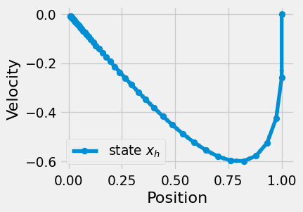
We see that the LQR control smoothly controls the position of the ball.
In this section, we’ll compute the optimal value function \(V^\star_h\), Q-function \(Q^\star_h\), and policy \(\pi^\star_h\) for an LQR problem (def. 3.5) using dynamic programming. The algorithm is identical to the one in Section 2.3.1, except here states and actions are vector-valued. Recall the definition of the optimal value function:
Definition 3.6 (Optimal value function in LQR) The optimal value function is the one that, at any time and in any state, achieves minimum cost across all policies \(\pi\) that are history-independent, time-dependent, and deterministic.
\[ \begin{aligned} V^\star_h(x) &= \min_{\pi} V^\pi_h(x) \\ &= \min_{\pi} \mathop{\mathbb{E}}_{\tau \sim \rho^\pi} \left[ \sum_{h'=h}^{H-1} \left( x_{h'}^\top Q x_{h'} + u_{h'}^\top R u_{h'} \right) \mid x_h= x \right] \\ \end{aligned} \tag{3.17}\]
Definition 3.7 (Optimal Q function in LQR) The optimal Q-function is defined in the same way, conditioned on the starting state-action pair:
\[ \begin{aligned} Q^\star_h(x, u) &= \min_{\pi} Q^\pi_h(x, u) \\ &= \min_{\pi} \mathop{\mathbb{E}}\left[ \sum_{h'=h}^{H-1}\left( x_{h'}^\top Q x_{h'} + u_{h'}^\top R u_{h'} \right) \mid x_h= x, u_h= u \right] \\ \end{aligned} \tag{3.18}\]
Remark 3.3 (Minimum over all policies). By Theorem 2.6, we do not lose any generality by only considering policies that are history-independent, time-dependent, and deterministic. That is, the optimal policy within this class is also globally optimal across all policies, in the sense that it achieves lower cost for any given trajectory prefix.
The solution has very simple structure: \(V_h^\star\) and \(Q^\star_h\) are upward-curved quadratics and \(\pi_h^\star\) is linear and furthermore does not depend on the amount of noise!
Theorem 3.2 (Optimal value function in LQR is an upward-curved quadratic) At each timestep \(h\in [H]\),
\[ V^\star_h(x) = x^\top P_hx+ p_h \tag{3.19}\]
for some symmetric, positive-definite \(n_x\times n_x\) matrix \(P_h\) and scalar \(p_h\in \mathbb{R}\).
Theorem 3.3 (Optimal policy in LQR is linear) At each timestep \(h\in [H]\),
\[ \pi^\star_h(x) = - K_hx \tag{3.20}\]
for some \(K_h\in \mathbb{R}^{n_u\times n_x}\). (The negative is due to convention.)
The construction (and inductive proof) proceeds similarly to the one in the MDP setting (Section 2.3.1). We leave the full proof, which involves a significant amount of linear algebra, to Section B.1.
graph RL
    Q0["$$Q^\star_{H-1} = r$$"] -- "$$\max_{a \in \mathcal{A}}$$" --> V0
    Q0 -- "$$\arg\max_{a \in \mathcal{A}}$$" --> P0["$$\pi^\star_{H-1}$$"]
    V0["$$V^\star_{H-1}$$"] -- "Bellman equations" --> Q1

    Q1["$$Q^\star_{H-2}$$"] -- "$$\max_{a \in \mathcal{A}}$$" --> V1
    Q1 -- "$$\arg\max_{a \in \mathcal{A}}$$" --> P1["$$\pi^\star_{H-2}$$"]
    V1["$$V^\star_{H-2}$$"] -- "Bellman equations" --> Q2

    Q2["..."]
Here we provide the concrete \(P_h, p_h\), and \(K_h\) used to compute the quantities above.
Definition 3.8 (Riccati equation) It turns out that the matrices \(P_0, \dots, P_{H-1}\) used to define \(V^\star\) obey a recurrence relation known as the Riccati equation:
\[ P_h= Q + A^\top P_{h+1} A - A^\top P_{h+1} B (R + B^\top P_{h+1} B)^{-1} B^\top P_{h+1} A, \tag{3.21}\]
where \(A \in \mathbb{R}^{n_x\times n_x}\) and \(B \in \mathbb{R}^{n_x\times n_u}\) are the matrices used to define the dynamics \(f\) and \(Q \in \mathbb{R}^{n_x\times n_x}\) and \(R \in \mathbb{R}^{n_u\times n_u}\) are the matrices used to define the cost function \(c\) (def. 3.5).
The scalars \(p_h\) obey the recurrence relation
\[ p_h= \mathrm{Tr}(\sigma^2 P_{h+1}) + p_{h+1} \tag{3.22}\]
and the matrices \(K_0, \dots, K_{H-1}\) for defining the policy satisfy
\[ K_h= (R + B^\top P_{h+1} B)^{-1} B^\top P_{h+1} A. \tag{3.23}\]
By setting \(P_H= 0\) and \(p_H= 0\),
def dp_lqr(A, B, Q, R, sigma, H):
    n_x, n_u = B.shape
    P = jnp.zeros(n_x, n_x)
    p = 0
    P_ary, p_ary = [], []
    for h in range(H):
        P = Q + A.T @ P @ A - A.T @ P @ B @ np.inv(R + B.T @ P @ B) @ B.T @ P @ A
        p = sigma ** 2 * np.trace(P) + p
        P_ary.append(P)
        p_ary.append(p)
    return reversed(P_ary), reversed(p)
Definition 3.9 (Dynamic programming in LQR) Let \(A, B, Q, R\) be the matrices that define the LQR problem, and let \(\sigma^2\) be the variance of the noise in the dynamics (def. 3.5).
Let’s consider how the state at time \(h\) behaves when we act according to this optimal policy. In the field of control theory, which is often used in high-stakes circumstances such as aviation or architecture, it is important to understand the way the state evolves under the proposed controls.
How can we compute the expected state at time \(h\) when acting according to the optimal policy? Let’s first express \(x_h\) in a cleaner way in terms of the history. Having linear dynamics makes it easy to expand terms backwards in time:
\[ \begin{aligned} x_h& = A x_{h-1} + B u_{h-1} + w_{h-1} \\ & = A (Ax_{h-2} + B u_{h-2} + w_{h-2}) + B u_{h-1} + w_{h-1} \\ & = \cdots \\ & = A^hx_0 + \sum_{i=0}^{h-1} A^i (B u_{h-i-1} + w_{h-i-1}). \end{aligned} \tag{3.24}\]
Let’s consider the average state at this time, given all the past states and actions. Since we assume that \(\mathop{\mathbb{E}}[w_h] = 0\) (this is the zero vector in \(d\) dimensions), when we take an expectation, the \(w_h\) term vanishes due to linearity, and so we’re left with
\[ \mathop{\mathbb{E}}[x_h\mid x_{0:(h-1)}, u_{0:(h-1)}] = A^hx_0 + \sum_{i=0}^{h-1} A^i B u_{h-i-1}. \tag{3.25}\]
Exercise 3.2 (Expected state) Show that if we choose actions according to the optimal policy Lemma B.2, eq. 3.25 becomes
\[ \mathop{\mathbb{E}}[x_h\mid x_0, u_i = \pi^\star_i(x_i)\quad \forall i \le h] = \left( \prod_{i=0}^{h-1} (A - B K_i) \right) x_0. \]
This introdces the quantity \(A - B K_i\), which shows up frequently in control theory. For example, one important question is: will \(x_h\) remain bounded, or will it go to infinity as time goes on? To answer this, let’s imagine for simplicity that these \(K_i\)s are equal (call this matrix \(K\)). Then the expression above becomes \((A-BK)^hx_0\). Now consider the maximum eigenvalue \(\lambda_{\max}\) of \(A - BK\). If \(|\lambda_{\max}| > 1\), then there’s some nonzero initial state \(\bar x_0\), the corresponding eigenvector, for which
\[ \lim_{h\to \infty} (A - BK)^h\bar x_0 = \lim_{h\to \infty} \lambda_{\max}^h\bar x_0 = \infty. \]
Otherwise, if \(|\lambda_{\max}| < 1\), then it’s impossible for your original state to explode as dramatically.
We’ve now formulated an optimal solution for the time-homogeneous LQR and computed the expected state under the optimal policy. However, real world tasks rarely have such simple dynamics, and we may wish to design more complex cost functions. In this section, we’ll consider more general extensions of LQR where some of the assumptions we made above are relaxed. Specifically, we’ll consider:
Combining these will allow us to use the LQR solution to solve more complex setups by taking Taylor approximations of the dynamics and cost functions.
So far, we’ve considered the time-homogeneous case, where the dynamics and cost function stay the same at every timestep. However, this might not always be the case. As an example, in many sports, the rules and scoring system might change during an overtime period. To address such tasks, we can loosen the time-homogeneous restriction, and consider the case where the dynamics and cost function are time-dependent. Our analysis remains almost identical; in fact, we can simply add a time index to the matrices \(A\) and \(B\) that determine the dynamics and the matrices \(Q\) and \(R\) that determine the cost.
The modified problem is now defined as follows:
Definition 3.10 (Time-dependent LQR) \[ \begin{aligned} \min_{\pi_{0}, \dots, \pi_{H-1}} \quad & \mathop{\mathbb{E}}\left[ \left( \sum_{h=0}^{H-1} (x_h^\top Q_hx_h) + u_h^\top R_hu_h\right) + x_H^\top Q_Hx_H\right] \\ \textrm{where} \quad & x_{h+1} = f_h(x_h, u_h, w_h) = A_hx_h+ B_hu_h+ w_h\\ & x_0 \sim \mu_0 \\ & u_h= \pi_h(x_h) \\ & w_h\sim \mathcal{N}(0, \sigma^2 I). \end{aligned} \]
The derivation of the optimal value functions and the optimal policy remains almost exactly the same, and we can modify the Riccati equation accordingly:
Definition 3.11 (Time-dependent Riccati Equation) \[ P_h= Q_h+ A_h^\top P_{h+1} A_h- A_h^\top P_{h+1} B_h(R_h+ B_h^\top P_{h+1} B_h)^{-1} B_h^\top P_{h+1} A_h. \]
Note that this is just the time-homogeneous Riccati equation (def. 3.8), but with the time index added to each of the relevant matrices.
Exercise 3.3 (Time dependent LQR proof) Walk through the proof in Section 3.4 to verify that we can simply add \(h\) for the time-dependent case.
Additionally, by allowing the dynamics to vary across time, we gain the ability to locally approximate nonlinear dynamics at each timestep. We’ll discuss this later in the chapter.
Our original cost function had only second-order terms with respect to the state and action, incentivizing staying as close as possible to \((x^\star, u^\star) = (0, 0)\). We can also consider more general quadratic cost functions that also have first-order terms and a constant term. Combining this with time-dependent dynamics results in the following expression, where we introduce a new matrix \(M_h\) for the cross term, linear coefficients \(q_h\) and \(r_h\) for the state and action respectively, and a constant term \(c_h\):
\[ c_h(x_h, u_h) = ( x_h^\top Q_hx_h+ x_h^\top M_hu_h+ u_h^\top R_hu_h) + (x_h^\top q_h+ u_h^\top r_h) + c_h. \tag{3.26}\]
Similarly, we can also include a constant term \(v_h\in \mathbb{R}^{n_x}\) in the dynamics. This is deterministic, unlike the stochastic noise \(w_h\):
\[ x_{h+1} = f_h(x_h, u_h, w_h) = A_hx_h+ B_hu_h+ v_h+ w_h. \]
Exercise 3.4 (General cost function) Derive the optimal solution. You will need to slightly modify the proof in Section 3.4.
Consider applying LQR to a task like autonomous driving, where the target state-action pair changes over time. We might want the vehicle to follow a predefined trajectory of states and actions \((x_h^\star, u_h^\star)_{h=0}^{H-1}\). To express this as a control problem, we’ll need a corresponding time-dependent cost function:
\[ c_h(x_h, u_h) = (x_h- x^\star_h)^\top Q (x_h- x^\star_h) + (u_h- u^\star_h)^\top R (u_h- u^\star_h). \]
Note that this punishes states and actions that are far from the intended trajectory. By expanding out these multiplications, we can see that this is actually a special case of the more general quadratic cost function above eq. 3.26:
\[ M_h= 0, \qquad q_h= -2Q x^\star_h, \qquad r_h= -2R u^\star_h, \qquad c_h= (x^\star_h)^\top Q (x^\star_h) + (u^\star_h)^\top R (u^\star_h). \]
The LQR algorithm solves for the optimal policy when the dynamics are linear and the cost function is an upward-curved quadratic. However, real settings are rarely this simple! Let’s return to the CartPole example from the start of the chapter (ex. 3.1). The dynamics (physics) aren’t linear. How can we approximate this by an LQR problem?
Concretely, let’s consider a noise-free problem since, as we saw, the noise doesn’t factor into the optimal policy. Let’s assume the dynamics and cost function are stationary, and ignore the terminal state for simplicity:
Definition 3.12 (Nonlinear control problem) \[ \begin{aligned} \min_{\pi_0, \dots, \pi_{H-1} : \mathcal{S} \to \mathcal{A}} \quad & \mathop{\mathbb{E}}_{x_0 \sim P_0} \left[ \sum_{h=0}^{H-1} c(x_h, u_h) \right] \\ \text{where} \quad & x_{h+1} = f(x_h, u_h) \\ & u_h= \pi_h(x_h) \\ & x_0 \sim \mu_0 \\ & c(x, u) = d(x, x^\star) + d(u, u^\star). \end{aligned} \]
Here, \(d\) denotes a function that measures the “distance” between its two arguments.
This is now only slightly simplified from the general optimal control problem (see def. 3.2). Here, we don’t know an analytical form for the dynamics \(f\) or the cost function \(c\), but we assume that we’re able to query/sample/simulate them to get their values at a given state and action. To clarify, consider the case where the dynamics are given by real world physics. We can’t (yet) write down an expression for the dynamics that we can differentiate or integrate analytically. However, we can still simulate the dynamics and cost function by running a real-world experiment and measuring the resulting states and costs. How can we adapt LQR to this more general nonlinear case?
How can we apply LQR when the dynamics are nonlinear or the cost function is more complex? We’ll exploit the useful fact that we can take a function that’s locally continuous around \((x^\star, u^\star)\) and approximate it nearby with low-order polynomials (i.e. its Taylor approximation). In particular, as long as the dynamics \(f\) are differentiable around \((x^\star, u^\star)\) and the cost function \(c\) is twice differentiable at \((x^\star, u^\star)\), we can take a linear approximation of \(f\) and a quadratic approximation of \(c\) to bring us back to the regime of LQR.
Linearizing the dynamics around \((x^\star, u^\star)\) gives:
\[ \begin{gathered} f(x, u) \approx f(x^\star, u^\star) + \nabla_xf(x^\star, u^\star) (x- x^\star) + \nabla_uf(x^\star, u^\star) (u- u^\star) \\ (\nabla_xf(x, u))_{ij} = \frac{d f_i(x, u)}{d x_j}, \quad i, j \le n_x\qquad (\nabla_uf(x, u))_{ij} = \frac{d f_i(x, u)}{d u_j}, \quad i \le n_x, j \le n_u \end{gathered} \]
and quadratizing the cost function around \((x^\star, u^\star)\) gives:
\[ \begin{aligned} c(x, u) & \approx c(x^\star, u^\star) \quad \text{constant term} \\ & \qquad + \nabla_xc(x^\star, u^\star) (x- x^\star) + \nabla_uc(x^\star, u^\star) (a - u^\star) \quad \text{linear terms} \\ & \left. \begin{aligned} & \qquad + \frac{1}{2} (x- x^\star)^\top \nabla_{xx} c(x^\star, u^\star) (x- x^\star) \\ & \qquad + \frac{1}{2} (u- u^\star)^\top \nabla_{uu} c(x^\star, u^\star) (u- u^\star) \\ & \qquad + (x- x^\star)^\top \nabla_{xu} c(x^\star, u^\star) (u- u^\star) \end{aligned} \right\} \text{quadratic terms} \end{aligned} \]
where the gradients and Hessians are defined as
\[ \begin{aligned} (\nabla_xc(x, u))_{i} & = \frac{d c(x, u)}{d x_i}, \quad i \le n_x & (\nabla_uc(x, u))_{i} & = \frac{d c(x, u)}{d u_i}, \quad i \le n_u\\ (\nabla_{xx} c(x, u))_{ij} & = \frac{d^2 c(x, u)}{d x_i d x_j}, \quad i, j \le n_x & (\nabla_{uu} c(x, u))_{ij} & = \frac{d^2 c(x, u)}{d u_i d u_j}, \quad i, j \le n_u\\ (\nabla_{xu} c(x, u))_{ij} & = \frac{d^2 c(x, u)}{d x_i d u_j}. \quad i \le n_x, j \le n_u \end{aligned} \]
Exercise 3.5 (Expressing as quadratic) Note that this cost can be expressed in the general quadratic form seen in eq. 3.26. Derive the corresponding quantities \(Q, R, M, q, r, c\).
To calculate these gradients and Hessians in practice, we use a method known as finite differencing for numerically computing derivatives. Namely, we can simply use the limit definition of the derivative, and see how the function changes as we add or subtract a tiny \(\delta\) to the input.
\[ \frac{d}{dx} f(x) = \lim_{\delta \to 0} \frac{f(x + \delta) - f(x)}{\delta} \]
This only requires us to be able to query the function, not to have an analytical expression for it, which is why it’s so useful in practice.
However, simply taking the second-order approximation of the cost function is insufficient, since for the LQR setup we required that the \(Q\) and \(R\) matrices were positive definite, i.e. that all of their eigenvalues were positive.
One way to naively force some symmetric matrix \(D\) to be positive definite is to set any non-positive eigenvalues to some small positive value \(\varepsilon > 0\). Recall that any real symmetric matrix \(D \in \mathbb{R}^{n \times n}\) has an basis of eigenvectors \(u_1, \dots, u_n\) with corresponding eigenvalues \(\lambda_1, \dots, \lambda_n\) such that \(D u_i = \lambda_i u_i\). Then we can construct the positive definite approximation by
\[ \widetilde{D} = \left( \sum_{i=1, \dots, n \mid \lambda_i > 0} \lambda_i u_i u_i^\top \right) + \varepsilon I. \]
Exercise: Convince yourself that \(\widetilde{D}\) is indeed positive definite.
Note that Hessian matrices are generally symmetric, so we can apply this process to \(Q\) and \(R\) to obtain the positive definite approximations \(\widetilde{Q}\) and \(\widetilde{R}\). Now that we have an upward-curved quadratic approximation to the cost function, and a linear approximation to the state transitions, we can simply apply the time-homogenous LQR methods from Section 3.4.
But what happens when we enter states far away from \(x^\star\) or want to use actions far from \(u^\star\)? A Taylor approximation is only accurate in a local region around the point of linearization, so the performance of our LQR controller will degrade as we move further away. We’ll see how to address this in the next section using the iterative LQR algorithm.
To address these issues with local linearization, we’ll use an iterative approach, where we repeatedly linearize around different points to create a time-dependent approximation of the dynamics, and then solve the resulting time-dependent LQR problem to obtain a better policy. This is known as iterative LQR or iLQR:
Definition 3.13 (Iterative LQR) For each iteration of the algorithm:
graph LR
    Approx["Locally approximate a linear model of the environment"] -- "$$f, c$$" --> Opt
    Opt["Solve for the optimal policy in the model"] -- "$$\pi^\star$$" --> Approx
Now let’s go through the details of each step. We’ll use superscripts to denote the iteration of the algorithm. We’ll also denote \(\bar x_0 = \mathop{\mathbb{E}}_{x_0 \sim \mu_0} [x_0]\) as the expected initial state.
At iteration \(i\) of the algorithm, we begin with a candidate trajectory \(\bar \tau^i = (\bar x^i_0, \bar u^i_0, \dots, \bar x^i_{H-1}, \bar u^i_{H-1})\).
Step 1: Form a time-dependent LQR problem. At each timestep \(h\in [H]\), we use the techniques from Section 3.6 to linearize the dynamics and quadratize the cost function around \((\bar x^i_h, \bar u^i_h)\):
\[ \begin{aligned} f_h(x, u) & \approx f(\bar {x}^i_h, \bar {u}^i_h) + \nabla_{x} f(\bar {x}^i_h, \bar {u}^i_h)(x- \bar {x}^i_h) + \nabla_{u} f(\bar {x}^i_h, \bar {u}^i_h)(u- \bar {u}^i_h) \\ c_h(x, u) & \approx c(\bar {x}^i_h, \bar {u}^i_h) + \begin{bmatrix} x- \bar {x}^i_h& u- \bar {u}^i_h \end{bmatrix} \begin{bmatrix} \nabla_{x} c(\bar {x}^i_h, \bar {u}^i_h)\\ \nabla_{u} c(\bar {x}^i_h, \bar {u}^i_h) \end{bmatrix} \\ & \qquad + \frac{1}{2} \begin{bmatrix} x- \bar {x}^i_h& u- \bar {u}^i_h \end{bmatrix} \begin{bmatrix} \nabla_{xx} c(\bar {x}^i_h, \bar {u}^i_h) & \nabla_{xu} c(\bar {x}^i_h, \bar {u}^i_h) \\ \nabla_{ux} c(\bar {x}^i_h, \bar {u}^i_h) & \nabla_{uu} c(\bar {x}^i_h, \bar {u}^i_h) \end{bmatrix} \begin{bmatrix} x- \bar {x}^i_h\\ u- \bar {u}^i_h \end{bmatrix}. \end{aligned} \]
Step 2: Compute the optimal policy. We solve the time-dependent LQR problem using the time-dependent algebraic Riccati equation (def. 3.11) to compute the optimal policy \(\pi^i_0, \dots, \pi^i_{H-1}\).
Step 3: Generate a new series of actions. We generate a new sample trajectory by taking actions according to this optimal policy:
\[ \bar x^{i+1}_0 = \bar x_0, \qquad \widetilde u_h= \pi^i_h(\bar x^{i+1}_h), \qquad \bar x^{i+1}_{h+1} = f(\bar x^{i+1}_h, \widetilde u_h). \]
Note that the states are sampled according to the true dynamics, which we assume we have query access to.
Step 4: Compute a better candidate trajectory. Note that we’ve denoted these actions as \(\widetilde u_h\) and aren’t directly using them for the next iteration \(\bar u^{i+1}_h\). Rather, we want to interpolate between them and the actions from the previous iteration \(\bar u^i_0, \dots, \bar u^i_{H-1}\). This is so that the cost will increase monotonically, since if the new policy turns out to actually be worse, we can stay closer to the previous trajectory. The new policy might be worse, for example, if the states in the new trajectory are far enough from the original states that the local linearization is no longer accurate.
Formally, we want to find \(\alpha \in [0, 1]\) to generate the next iteration of actions \(\bar u^{i+1}_0, \dots, \bar u^{i+1}_{H-1}\) such that the cost is minimized:
\[ \begin{aligned} \min_{\alpha \in [0, 1]} \quad & \sum_{h=0}^{H-1} c(x_h, \bar u^{i+1}_h) \\ \text{where} \quad & x_{h+1} = f(x_h, \bar u^{i+1}_h) \\ & \bar u^{i+1}_h= \alpha \bar u^i_h+ (1-\alpha) \widetilde u_h\\ & x_0 = \bar x_0. \end{aligned} \]
Note that this optimizes over the closed interval \([0, 1]\), so by the Extreme Value Theorem, it’s guaranteed to have a global maximum.
The final output of this algorithm is a policy \(\pi^{n_\text{steps}}\) derived after \(n_\text{steps}\) of the algorithm. Though the proof is somewhat complex, one can show that for many nonlinear control problems, this solution converges to a locally optimal solution (in the policy space).
This chapter introduced some approaches to solving simple variants of the optimal control problem def. 3.2. We began with the simple case of linear dynamics and an upward-curved quadratic cost. This model is called the linear quadratic regulator (LQR). The optimal policy can be solved using dynamic programming. We then extended these results to the more general nonlinear case via local linearization. We finally studied the iterative LQR algorithm for solving nonlinear control problems.
In the big picture, the LQR algorithm can be seen as an extension of the dynamic programming algorithms in Chapter 2 to continuous state and action spaces. Both of these methods assume that the environment is fully known. iLQR loosens this assumption slightly: as long as we have “query access” to the environment, that is, we can efficiently sample the state following any given state-action pair, we can locally approximate the dynamics using finite differences.
The field of control theory generally predates that of RL and can be seen as a precursor to the model-based planning algorithms used for RL tasks. People have attempted to solve the optimal control problem since antiquity: the first recorded control device (i.e. our notion of a policy, put into practice) is thought to be a water clock from the third century BCE that kept time by controlling the amount of water flowing out of a vessel (Keviczky et al., 2019; Mayr, 1970).
Watt’s 1788 centrifugal governor for controlling the pace of a steam engine was one of the greatest inventions in control at the time. We refer the reader to (Bellman, 1961; MacFarlane, 1979) for more on the history of control systems.
The first attempt to formalize control theory as a field is attributed to Maxwell (1867). Maxwell (well known for Maxwell’s equations) demonstrated the utility of analyzing mathematical models to design stable systems. Other researchers also studied the stability of differential equations. The work of Lyapunov (1892) has been widely influential in this field; his seminal work did not appear in English until Ljapunov & Fuller (1992).
A number of excellent textbooks have been published on optimal control (Athans & Falb, 1966; Bellman, 1957; Berkovitz, 1974; Lewis et al., 2012). We refer interested readers to these for further reading, particularly about the continuous-time case.